DASoftware

============

This is a Matlab library of data assimilation methods developed to solve large-scale state-parameter estimation problems. Data assimilation approach has been widely used in geophysics, hydrology and numerical weather forecast to improve the forecast from a numerical model based on data sets collected in real time. Conventional approach like Kalman filter is computatioanlly prohibitive for large problems. The DASoftware library takes advantage of advances in computatioanl science and consists of new data assimilation approach that is scalable for large-scale problems. The functions and examples are produced based on collabrated work on data assimialtion documented in the papers listed in the Reference section.

This is an ongoing project. The library is incomplete.

Highlight

Data assimilation tools for Large-scale real-time estimation problems

Computationally efficient methods with linear complexity(O(m)) that runs fast even on laptops

Hands-on examples to learn Kalman filters without the knowledge of the technical details

Summary of Example

Example	Dimension	Linearity	Specific
Saetrom	1D	Linear	F(x,t)
Target tracking	1D	Nonlinear	F(x),H(x)
Frio	2D	Linear	F = I, fixed H

Summary of methods

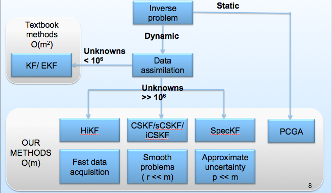
Here we show a diagram of the methods provided in the library.

Method	Assumptions	Jacobian matrix	Covariance matrix
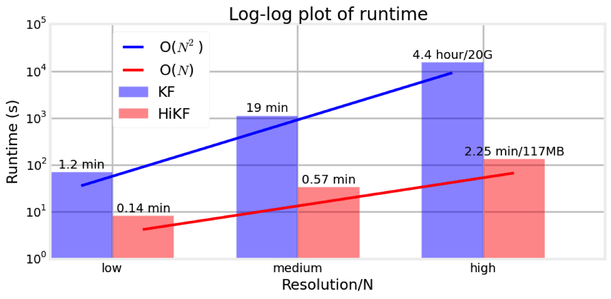
KF	only for small problem	mn forward run	m^2 operations
HiKF	fast data acquisition/fixed H	no forward run	O(m) operations
	random-walk forward model
CSKF	smooth problem	r forward run	O(m) operations
SpecKF	approximate uncertainty/fixed H	p forward run	O(m) operations
EnKF	monte carlo based approach	r forward run	O(m) operations

Quick Start Guide

To get you up and running DASoftware

Prerequisites

This Quick Start Guide assumes that you have the following already installed:

mexBBFMM2D: see the Quick Start Guide for mexBBFMM2D for installing MEX and other dependent libraries. This library is required to run Frio example.
git: a version control tool

Start with examples

Download the package by entering the following code in your command line

git clone https://github.com/judithyueli/DASoftware.git

Obtain data from here and put it in the directory /DASoftware/data

We have provided the users linear and nonlinear state estimation problems to get familier with data assimilation methods provided in the library. All the built-in examples can be operated using a simple one-line code with an input file (*.txt) including all the assimilation parameters. To run an example, go to the main folder /DASoftware containing main.m and type the following code in MATLAB

[est,true,est_array,true_array] = main(example_txt_file_name);

Input:

example_txt_file_name is the name of the input text file under the folder \example containing the following field

method: name of the Kalman filter method, e.g., KF, CSKF, HiKF
model: name of the built in example, e.g., Saetrom, TargetTracking, Frio
m: number of unknown state variables
n: number of observed variables
nt: total assimialtion time steps
x_std: initial state standard deviation
cov_type: state covariance type, e.g., exponential, Gaussian, state covariance is specified through a covariance function with two hyperparameters, i.e., power given by cov_power and length scale given by cov_len
BasisType: a field required for method CSKF specifying the dimension reduction type, e.g., the randomized SVD approach rSVD
mexBBFMM: optional for the Frio example. If mexBBFMM = 1 a fast linear algebraic package is used to accelerate the Kalman filter. Default is 0

Output:

est: an object containing the Kalman filter estimate at the final assimilation step. Visit the class definition for more information.

est.x: a structure containing the value of the estimated state as a vector
est.P: the covariance matrix at the final assimilation step

true: an object containing the properties of the true state at the final assimilation step. Visit the class definition for more information.

true.xt: a structure containing the value of the true state as a vector
true.zt: a structure containing the true observation as a vector

est_array: a cell array of structures containing the estimated state given by Kalman filter at each assimilation step

true_array: a cell array of structures containing the true state at each assimilation step

1D Saetrom example

Run a 1-D linear state estimation example (Sætrom & Omre 2011) with Kalman filter

[est,true,est_array,true_array]=main('examples/prm-saetrom-KF.txt');

Example of user specified input in prm-saetrom-KF.txt

method          KF
model           Saetrom
m               100
n               13
nt              10
x_std           20
obsstd          1
cov_type        exponential
cov_power       1
cov_len         6
seed            10

Figure shows the mean and 95% confidence interval at intial and final time step.

Run the same problem using CSKF (Li et al. 2015) with N = 20 basis

[est,true,est_array,true_array]=main('examples/prm-saetrom-CSKF.txt');

Example of user specified input in prm-saetrom-CSKF.txt

method          CSKF
model           Saetrom
N               20
BasisType       rSVD
m               100
n               13
nt              10
x_std           20
obsstd          1
cov_type        exponential
cov_power       1
cov_len         6
seed            10

Target tracking example

Consider tracking an aircraft with an unknown constant maneuvering rate using a radar sensor (angle and bearing) yields a model with nonlinear dynamical and measurement equation. The unknown is the location, velocity and the turing rate.

[est,true,est_array,true_array]=main('examples/prm-target-KF.txt');

Example of user specified input in prm-target-KF.txt

model           TargetTracking
rate            3
dt              1
method          KF
nt        	    100
seed            200
theta_Q         0.6
theta_R         0.3

Frio example

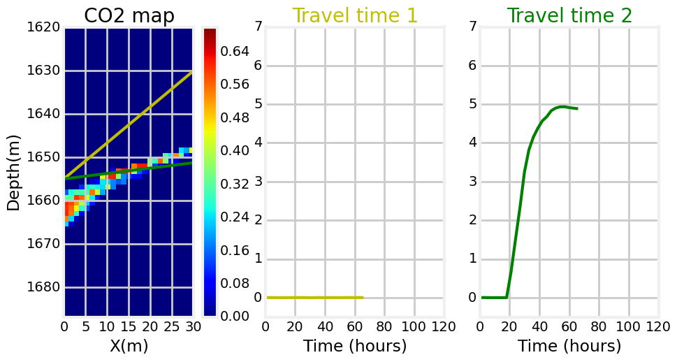
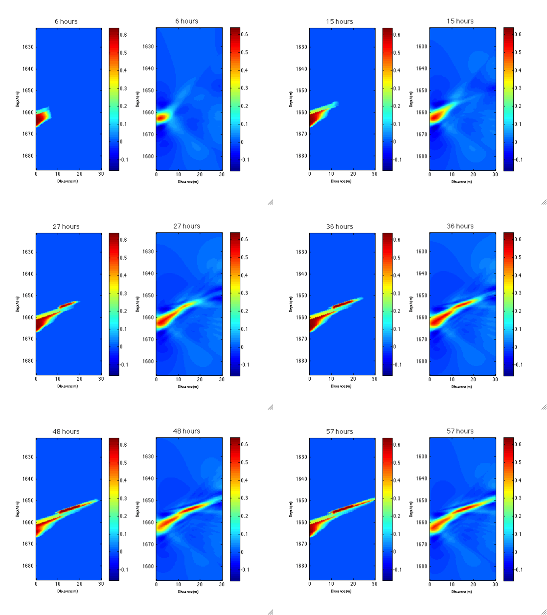
A description of this example can be found in Daley et al., 2011 and Li et al., 2014. Figure below shows how traveltime time-series signals recorded by sensors at different location can be used to constrain the position of a moving CO2 plume. With the computational efficiency provided by methods like HiKF, these sensor data can be processed in real-time to monitor potential CO2 leakage.

[est,true,est_array,true_array]=main('examples/prm-Frio-HiKF.txt');

Example of user specified input for a low resolution case containing 3245 unknowns.

method          HiKF
model           Frio
resolution      low
nt              40
theta_Q         1.14e-7
theta_R         1e-5
cov_type    	exponential
cov_power      	0.5
cov_len         900
seed            100
mexBBFMM        0
mexfile_name    expfun

To run a higher resolution case containing 12753 unknowns, run the following code, this may take a few minutes to compile

[est,true,est_array,true_array]=main('examples/prm-Frio-HiKF-M.txt');

Details of the prm-Frio-HiKF.txt. Note that mexBBFMM = 1 in order to call the mexBBFMM2D package.

method          HiKF
model           Frio
resolution      medium
nt              40
theta_Q         1.14e-7
theta_R         1e-5
cov_type    	exponential
cov_power      	0.5
cov_len         900
seed            100
mexBBFMM        1
mexfile_name    expfun

Reference:

Judith Yue Li, Sivaram Ambikasaran, Eric F. Darve, Peter K. Kitanidis, A Kalman filter powered by H2-matrices for quasi-continuous data assimilation problems link
Sivaram Ambikasaran, Judith Yue Li, Peter K. Kitanidis, Eric Darve, Large-scale stochastic linear inversion using hierarchical matrices, Computational Geosciences, December 2013, Volume 17, Issue 6, pp 913-927 link
Ghorbanidehno, H., A. Kokkinaki, J. Y. Li, E. Darve, and P. K. Kitanidis, 2014. Real time data assimilation for large-scale systems with the Spectral Kalman Filter: An application in CO2 storage monitoring, Submitted to Advances in Water Resources, Special issue on data assimilation (under review)
Judith Yue Li, A. Kokkinaki, H. Ghorbanidehno, E. Darve, and P. K. Kitanidis, 2015. The nonlinear compressed state Kalman filter for efficient large-scale reservoir monitoring, Submitted to Water Resources Research (under review)
Sætrom, J., & Omre, H. (2011). Ensemble Kalman filtering with shrinkage regression techniques. Computational Geosciences, 15(2), 271–292.
Daley, Thomas M and Ajo-Franklin, Jonathan B and Doughty, Christine, 2011. Constraining the reservoir model of an injected CO2 plume with crosswell CASSM at the Frio-II brine pilot, International Journal of Greenhouse Gas Control, 5(4), 1022-1030.

Acknowledgement

We want to thank Dr Jonanthan Ajo-Franklin for providing us part of the data of Frio example.

linix100/DASoftware