# Install sml
library(devtools);
install_github('linxihui/sml');Cox's model assumes that the proportional hazards are proportional among all observations. With such assumption, a partial likelihood comes up, which can also be treated as a profile and conditional likelihood, which does not involve a baseline hazard function, and thus parameters of interest gain more degree freedom to estimate.
The Cox partial likelihood looks like
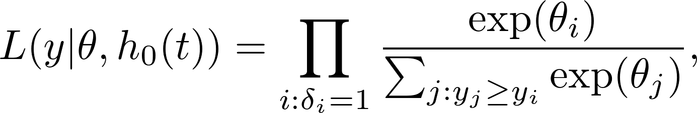
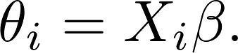
where
In Cox's model,
Gaussian process regression and classification have been shown to be powerful. However, no extension to survival
is available in R. However, the extension is quite straight forward, by assuming that
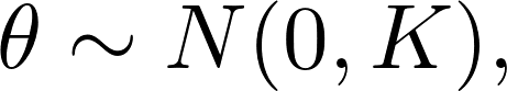
where
The posterior distribution,

Define

After taking the logarithm, we get

The max-a-posterior(MAP) estimate
# Survival Gaussian process regression

library(survival);
library(sml);
set.seed(123);
data(pbc, package = 'randomForestSRC');
pbc <- na.omit(pbc);
i.tr <- sample(nrow(pbc), 100);

gp <- gpsrc(Surv(days, status) ~., data = pbc[i.tr, ], kernel = 'laplacedot');
gp.pred <- predict(gp, pbc[-i.tr, ]);
gp.cInd <- survConcordance(Surv(days, status) ~ gp.pred, data = pbc[-i.tr, ]);
cat('C-index:', gp.cInd$concordance, '\n');
## C-index: 0.8492154
Extreme learning machine (ELM) was first introduced as a quick method to train a single hidden layer neural network. However, ELM is more related to SVM. Indeed, neural network trained to learn the hidden features and SVM maps input to high dimension feature space which is determinant. Instead, ELM randomly maps input to high dimension feature space. This random feature mapping turns out to work well.
Denote
Usually,
The question is, why random mapping even works? Since usually
![]()
almost surely. However, after applying a non-linear activating function,
![]()
# Survival ELM

elm.f <- elm(Surv(days, status) ~., data = pbc[i.tr, ], nhid = 500);
elm.pred <- predict(object = elm.f, newdata = pbc[-i.tr, ], type = 'link');
elm.cInd <- survConcordance(Surv(days, status) ~ elm.pred, data = pbc[-i.tr, ]);
cat('C-index:', elm.cInd$concordance, '\n');
## C-index: 0.839515
Let
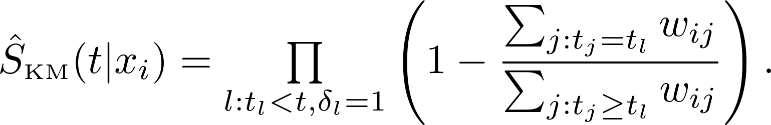
The weighted Nelson-Aalen estimator for the cummulative hazard function is
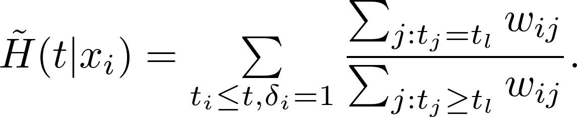
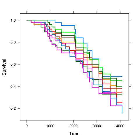
# Kernel-weighted KNN Kaplan-Meier

kkm.pred <- kkm(
	Surv(days, status) ~., data = pbc[i.tr, ], xtest = pbc[-i.tr, ],
	kernel = 'laplacedot', kpar = list(sigma = 0.1), k = 50
	);
kkm.cInd <- survConcordance(
	Surv(days, status) ~ I(1 - kkm.pred$test.predicted.survival[, 30]),
	data = pbc[-i.tr, ]
	);
cat('C-index:', kkm.cInd$concordance, '\n');
plot(kkm.pred, subset = sample(length(i.tr), 10), lwd = 2);
## C-index: 0.8446505