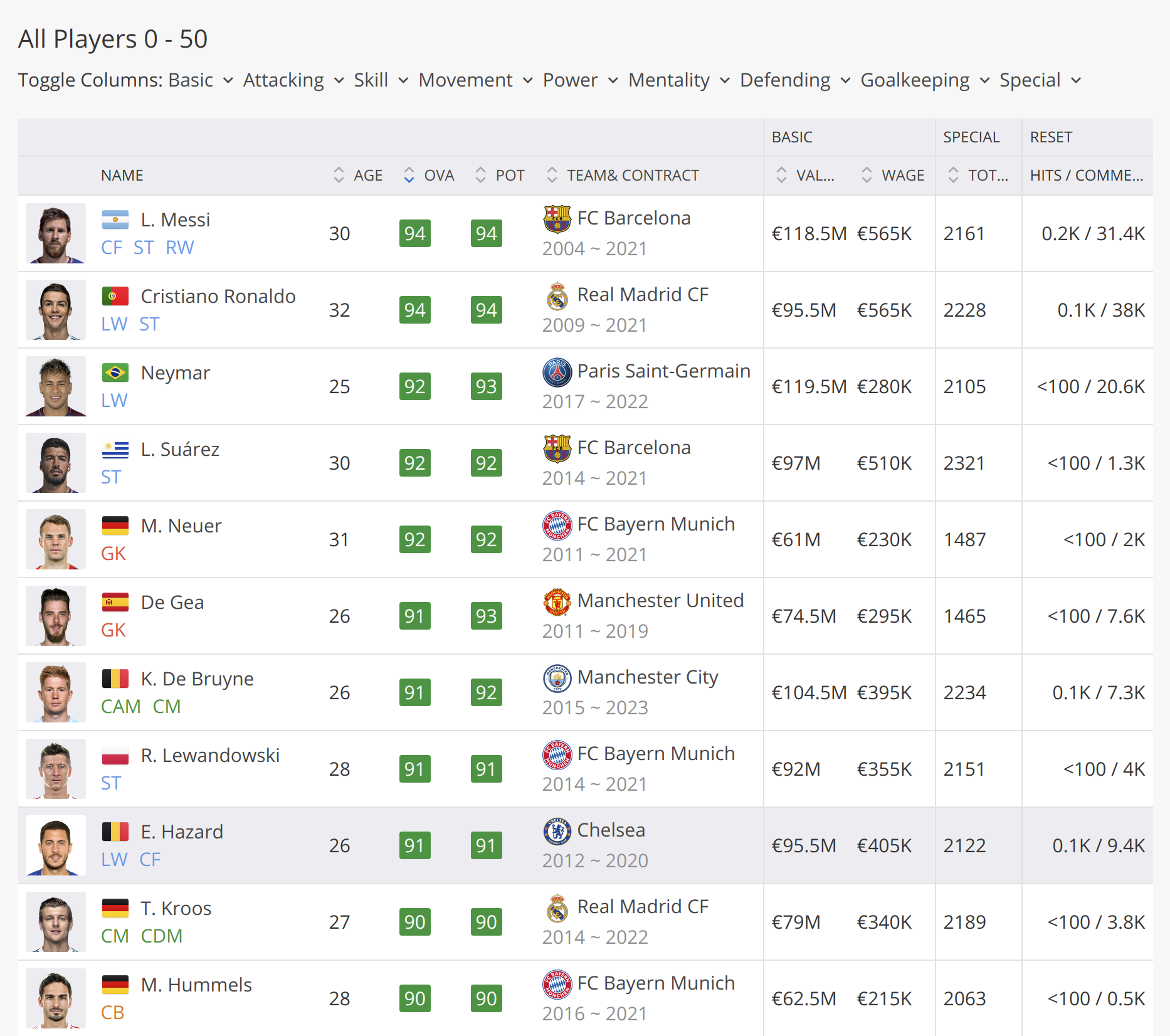
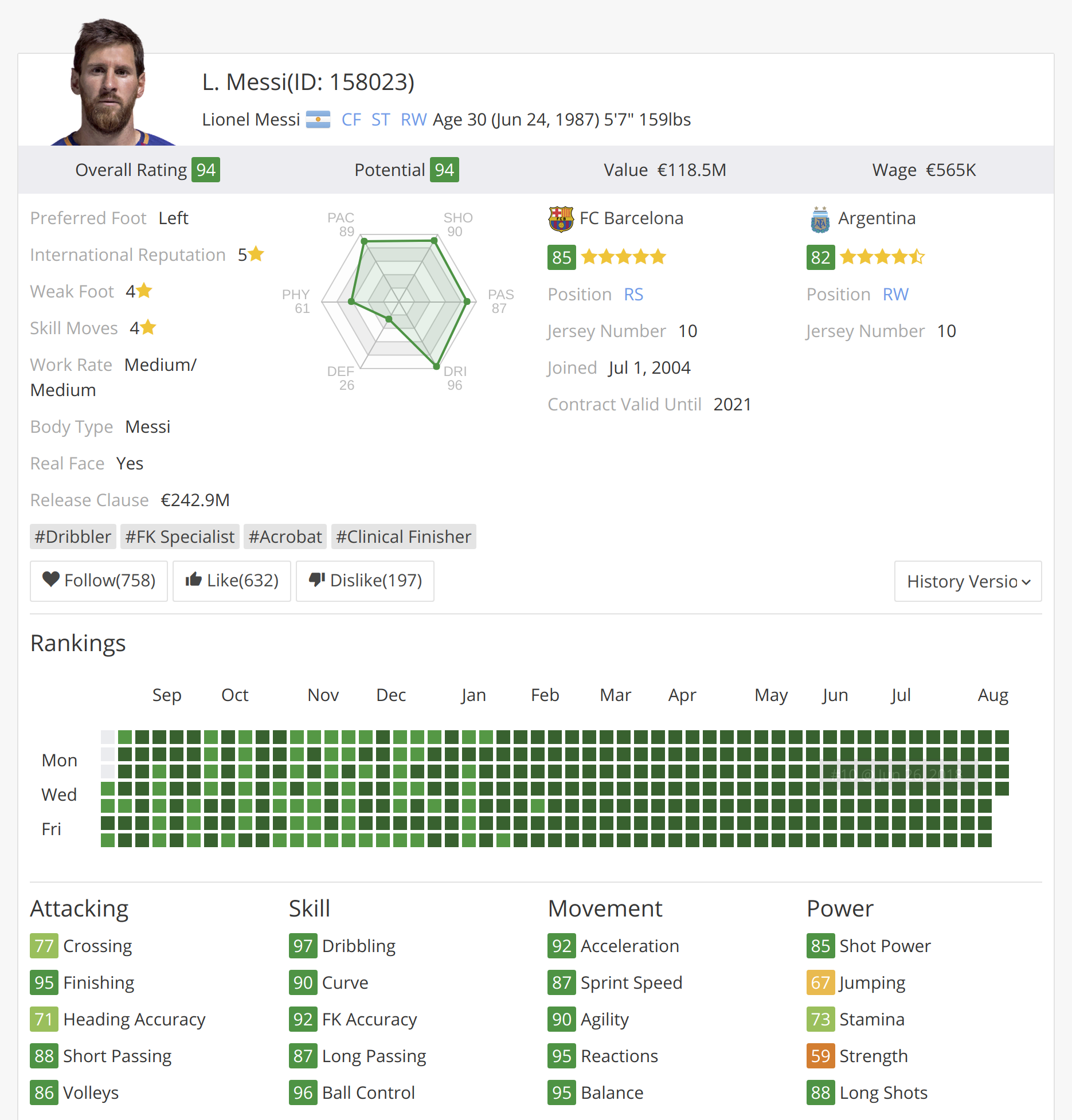
The Dataset you can play with.
Dataset for people who love data science and have grown up playing FIFA.
- Every player featuring in FIFA 18
- 70+ attributes
- Player and Flag Images
- Playing Position Data
- Attributes based on actual data of the latest EA's FIFA 18 game
- Attributes include on all player style statistics like Dribbling, Aggression, GK Skills etc.
- Player personal data like Nationality, Photo, Club, Age, Wage, Salary etc.
Upcoming Update will Include :
- Team (National and Club) Data
- Player Images in Zip folder
- Betting Odds
The dataset contains all the statistics and playing attributes of all the players in the Full version of FIFA 18.
The data is scraped from the website https://sofifa.com by extracting the Player personal data and Player Ids and then the playing and style statistics.
- Make your dream team
- Analyse which Club or National Team has the best-rated players
- Assess the strength of a team at a particular position
- Analyse the team with the best dribbling speed
- Co-relate between Age and Overall rating
- Co-relate between Age and Nationality
- Co-relate between Age and Potential
Could prove of immense value to Fantasy Premier League enthusiasts.
These are just basic examples, sky is the limit.
The data has been crawled from the https://sofifa.com website.
Several insights and correlations between player value, wage, age, and performance can be derived from the dataset. Furthermore, how do the players in this dataset compare against themselves in last year's dataset?
The project is for people who love data science and have grown up playing football and are FIFA enthusiasts. The data is scraped from the website https://sofifa.com by extracting the Player personal data, followed by Player IDs and their playing and style statistics.
Insights and correlations between player value, wage, age, special attributes, and performance can be derived from the dataset. This uninterpreted data can be converted into information by analysing it. We have derived summary statistics for teams, clubs, & players. Through extensive football experience: the insights provided in our results, alongwith understanding, and contextualized information enables users to act smartly when playing FIFA, picking a better team for say Fantasy Premier league, or increase their betting odds.
- World statistics
- Clustering players by Nationality
- Value & Wages of players with age
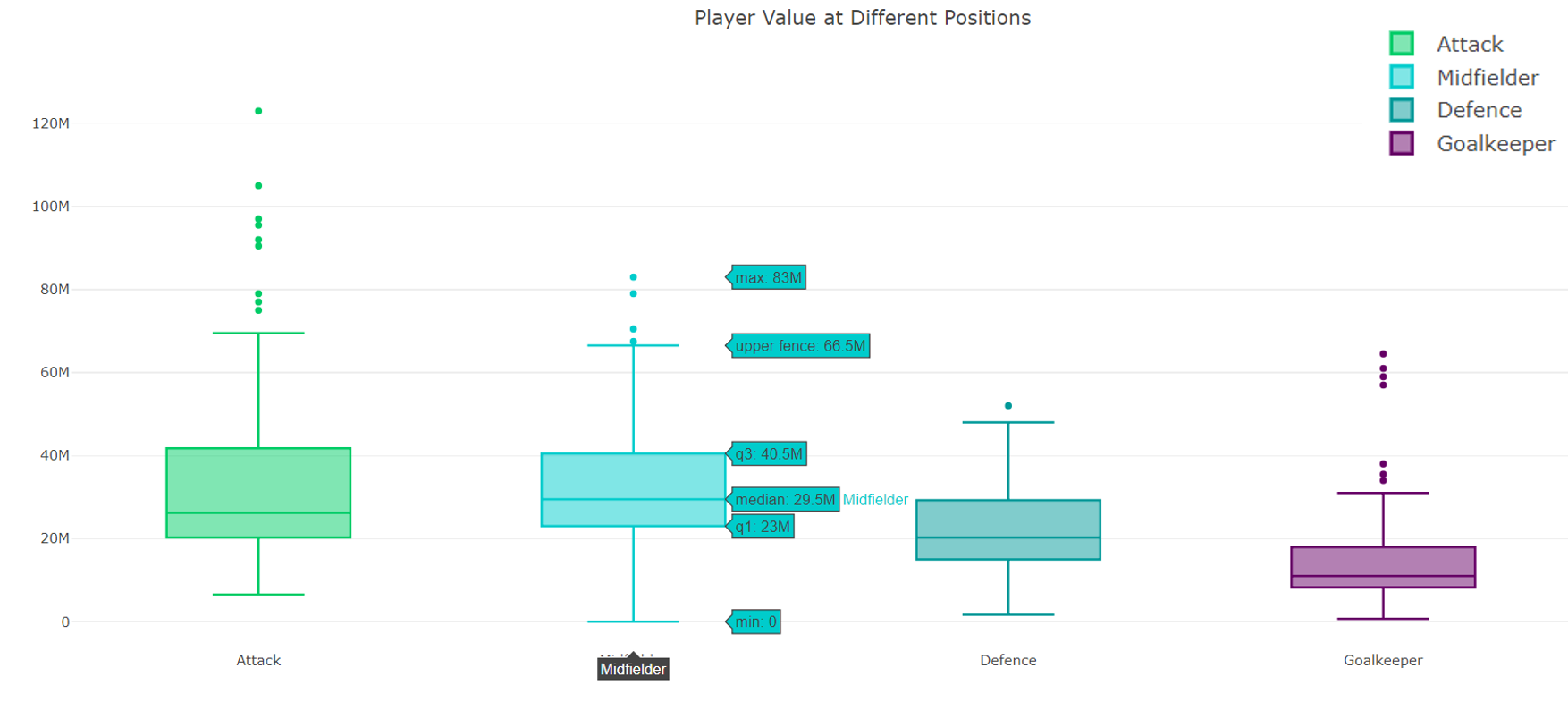
- Value of players with position
- Overall & Potential with age
- Variation of overall & potential by country for top countries
- Correlation matrix - attributes vs potential and overall
- Variation in wages for top clubs
- Age vs overall clustered by field position
- Make your dream team
- Predicting playing position using player statistics
The data was scrapped from the sofifa website using a python crawling script. The website contains the data from the EA Sports' game FIFA and gets updated regularly with the release of new versions of the game. data developed by Electronic Arts for the latest edition of their FIFA game franchise. Through several research projects done on soccer analytics, it has been established in the field of academia that the use of data from the FIFA franchise has several merits that traditional datasets based on historical data do not offer. Since 1995 the FIFA Soccer games provide an extensive and coherent scout of players worldwide.
For each attribute, we have an integer from 0 to 100 that measures how good a player is at that attribute. Examples of attributes are: dribbling, aggression, vision, marking and ball control. Observe that it seems to be unfeasible to accurately characterize players in these attributes automatically. Thus, all of those are gathered and curated by the company whose job is to bring the gameplay closer to reality as possible, hence preserving coherence and representativeness across the dataset.
The FIFA 18 dataset that has been used for this analysis provides statistics of about 16000 players on over 70 different attributes. These attributes are optimal indicators to determine the performance of a player at a particular playing position.
After extensively studying the structure of the website, the crawler was designed to scrape the website in two steps. The first step was to scrape the main page of the webpage which contains basic player information in a table. Apart from extracting the basic player info the crawler extracted the url of the player's detailed statistics page.
The table on the webpage had entries for 80 players on each page and the url of the page took offset for player id as a query parameter. The scrapper managed to algorithmically generate the urls of all the pages on website by manipulating the offset query in the url and iteratively visited all the pages to extract the details.
The next step was to use the collected urls for individual players to scrape data from their details page. This page contained skill statistics, team affiliations and performance statistics for the player.
The scrapped dataset has the following properties:
- Every player featuring in FIFA 18
- 70+ attributes
- Player and Flag Images
- Playing Position Data
- Attributes based on actual data of the latest EA's FIFA 18 game
- Attributes include on all player style statistics like Dribbling, Aggression, GK Skills etc.
- Player personal data like Nationality, Photo, Club, Age, Wage, Salary etc.
data.columns
Index(['ID', 'Photo', 'Name', 'Age', 'Nationality', 'Flag', 'Overall',
       'Potential', 'Club', 'Club Logo', 'Value', 'Wage', 'Special',
       'Acceleration', 'Aggression', 'Agility', 'Balance', 'Ball control',
       'Composure', 'Crossing', 'Curve', 'Dribbling', 'Finishing',
       'Free kick accuracy', 'GK diving', 'GK handling', 'GK kicking',
       'GK positioning', 'GK reflexes', 'Heading accuracy', 'Interceptions',
       'Jumping', 'Long passing', 'Long shots', 'Marking', 'Penalties',
       'Positioning', 'Reactions', 'Short passing', 'Shot power',
       'Sliding tackle', 'Sprint speed', 'Stamina', 'Standing tackle',
       'Strength', 'Vision', 'Volleys', 'CAM', 'CB', 'CDM', 'CF', 'CM', 'LAM',
       'LB', 'LCB', 'LCM', 'LDM', 'LF', 'LM', 'LS', 'LW', 'LWB',
       'Preferred Positions', 'RAM', 'RB', 'RCB', 'RCM', 'RDM', 'RF', 'RM',
'RS', 'RW', 'RWB', 'ST'], dtype='object')As the data was scrapped from a website it had several inconsistencies and properties that made it unfit for appropriate exploratory analysis. In order to prepare the data, the following steps were performed:
- The Wage and Value of all the players were in form of strings with the symbol of the currency in front of the values -
€190K. These had to converted to numeric values. - The preferred positions of all the players was available as a space separated string (
ST LW) which was converted to a list for easier retrieval. - A new attribute
FieldPositionwas created by mapping the preferred positions of all the players with their respective roles in the team, like attack, midfielder, defence or goalkeeper. - Using the nationality of the players, a new attribute was created that contained the continent the player belonged to.
After preparing the dataset for analysis, explorations were made on a macro level like continent and player nationality level analysis as well as on player level. Through the process attempts were made to derive interesting correlations and trends by the use of visualizations.
Circle-packing is the arrangement of circles inside some demarcation so that none of the circles overlap. Circle packing also displays hierarchy where you can get smaller clusters of circles packed within a bigger circle which itself is arranged next to or within other circles. The D3.js plot will be interactive and dynamic, where one is able to invoke zoomable animations at different regions and clusters with the click of a mouse button. The D3.js plot will be interactive and dynamic, where one is able to invoke zoomable animations at different regions and clusters with the click of a mouse button. Each of the player’s nationality was mapped to its respective continent. There were 162 distinct Nationality values in the dataset and these countries were mapped to 6 continents: Asia, Europe, Africa, North America, South America and Australia/Oceania. In the plot, the 6 continents will be the parent class (outer circles). We can dive deeper within this class to find the countries (sub-class / sub-circles) and within each country, we will find the players (inner circles). The size of the player circle is determined by the Overall variable. A continent dictionary was created with the names of the continents as the keys and the list of countries as the values for each key. A function was defined to assign the continent for each country. The top 2000 players were chosen based on the overall value. Groupings of the players were hence identified using the Nationality and Continent. This grouping will be displayed with the circle graph plot and is fed into the json file. The data to be displayed is stored in the json file.
This plot clearly shows the concentration of players across the continents. The size of the circles determines the number of top players in each region. Most of the top players are concentrated in Europe and South America. These two circles are significantly bigger than the other circles. Africa, Asia and North America have only few top players compared to Europe and South America though they are bigger in terms of size. This is clearly seen from the size of the circles. In Europe, Spain, Germany, France, Italy and Portugal have a very good number of top players. For South America, it is Brazil and Argentina. The distribution of top players across regions is useful in predicting the best team according to Nationality.
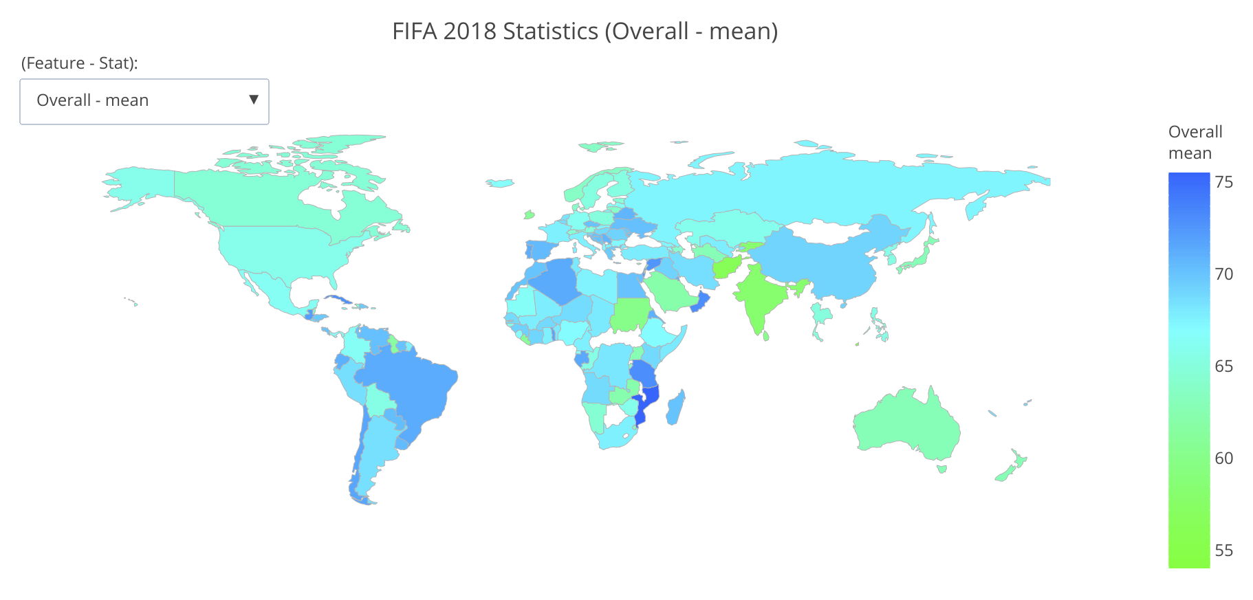
This section explores aggregate statistics of players hailing from all major football playing nations. Country wise mean, maximum and minimum values were identified for all the numeric attributes and plotted on an interactive world map.
The above plot demonstrates that South American, African and European players are generally rated higher than their counterparts from Asia, Australia or North America. While the nationwide average rating for USA stands at 65.81 and 58.06 for India it is about 71.24 for Brazil and 69.11 for China.
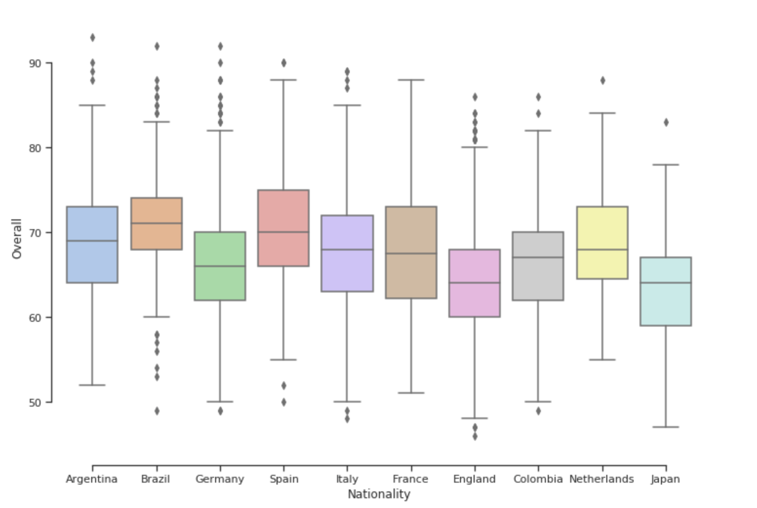
To explore which teams have the potential to surpass the current best, the following analysis was done. The top 10 countries by number of players were chosen and the overall and potential of their players were depicted as box plots.
| Overall Rating | Potential Rating |
|---|---|
 |
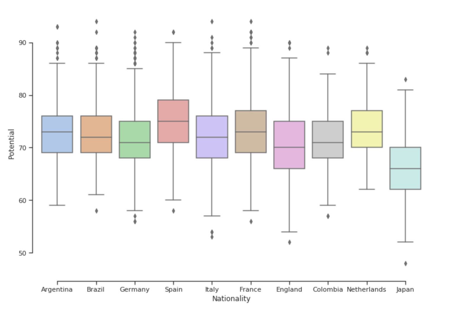 |
The mean overall is seen to be highest for Brazil followed by Spain, Argentina, Netherlands and France. However, in terms of potential, Spain seems to have overtaken Brazil, followed by Netherlands and France. This gives an indication about which teams are likely to perform better in the coming few years. Further ways in which this analysis can be improved is by plotting box plots against the highly and mildly correlated attributes that we saw above to reveal which are the attributes a country’s players are focusing on and make changes in their strategy if deemed fit.
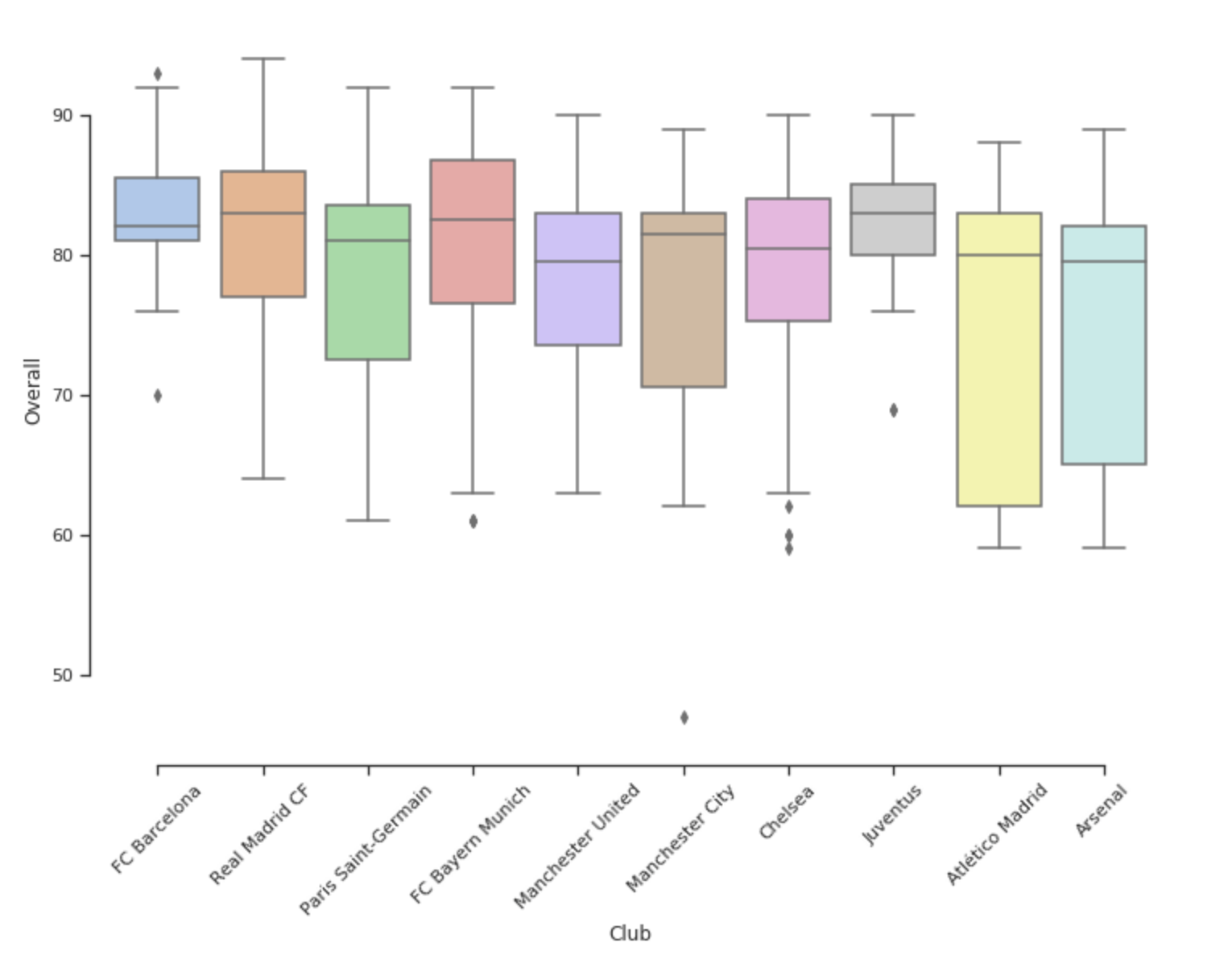
The aggregate overall and potential rating were compared among and between the top 10 football clubs. These clubs were identified to have the best overall rating aggregate.
| Club | Average Rating |
|---|
Real Madrid CF | 83.0
Juventus |	83.0
FC Bayern Munich |	82.5
FC Barcelona |	82.0
Manchester City |	81.5
Paris Saint-Germain |	81.0
Chelsea |	80.5
Atlético Madrid|	80.0
Manchester United|	79.5
Arsenal |	79.5
The variation of overall rating and potential rating was then demonstrated for these clubs using boxplots. This gives an indication about which teams are likely to perform better in the coming few years. Further ways in which this analysis can be improved is by plotting box plots against the highly and mildly correlated attributes that we saw above to reveal which are the attributes a country’s players are focusing on and make changes in their strategy if deemed fit.
| Overall Rating | Potential Rating |
|---|---|
 |
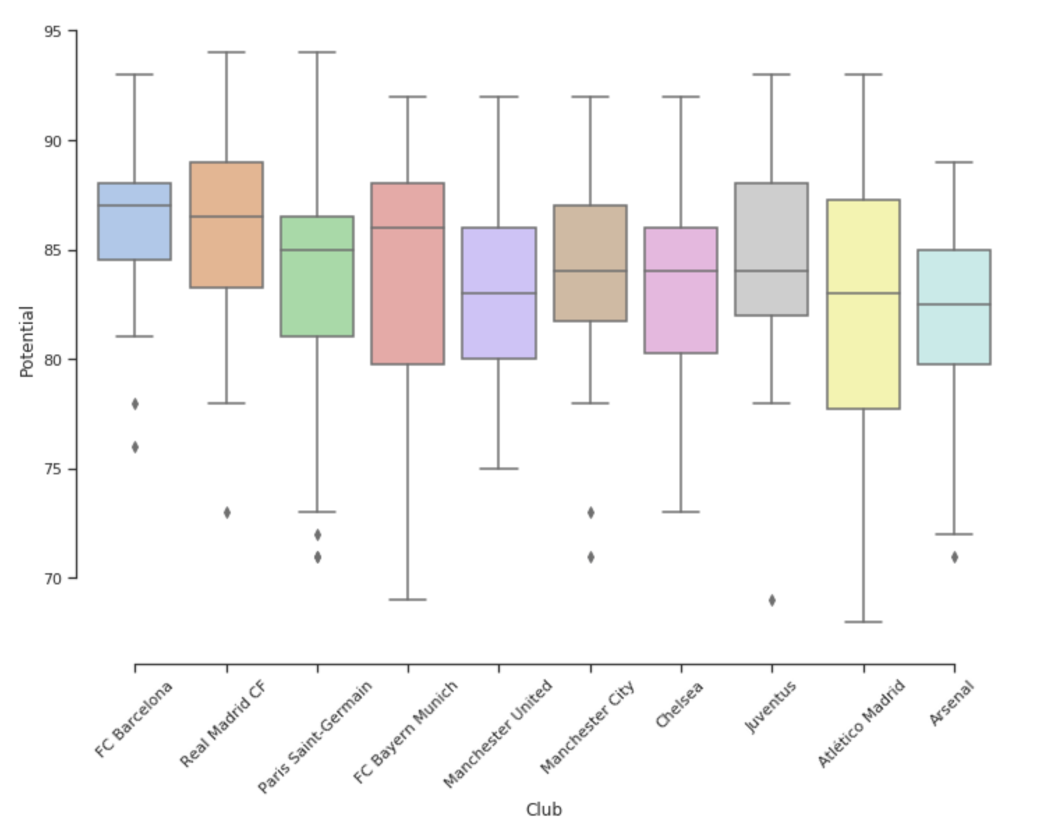 |
The mean overall is seen to be highest for Real Madrid followed by Juventus, FC Bayern Munich, FC Barcelona and Manchester City. However, in terms of potential, FC Barcelona seems to have overtaken Real Madrid, indicating a presence of a lot of young talent at the club.
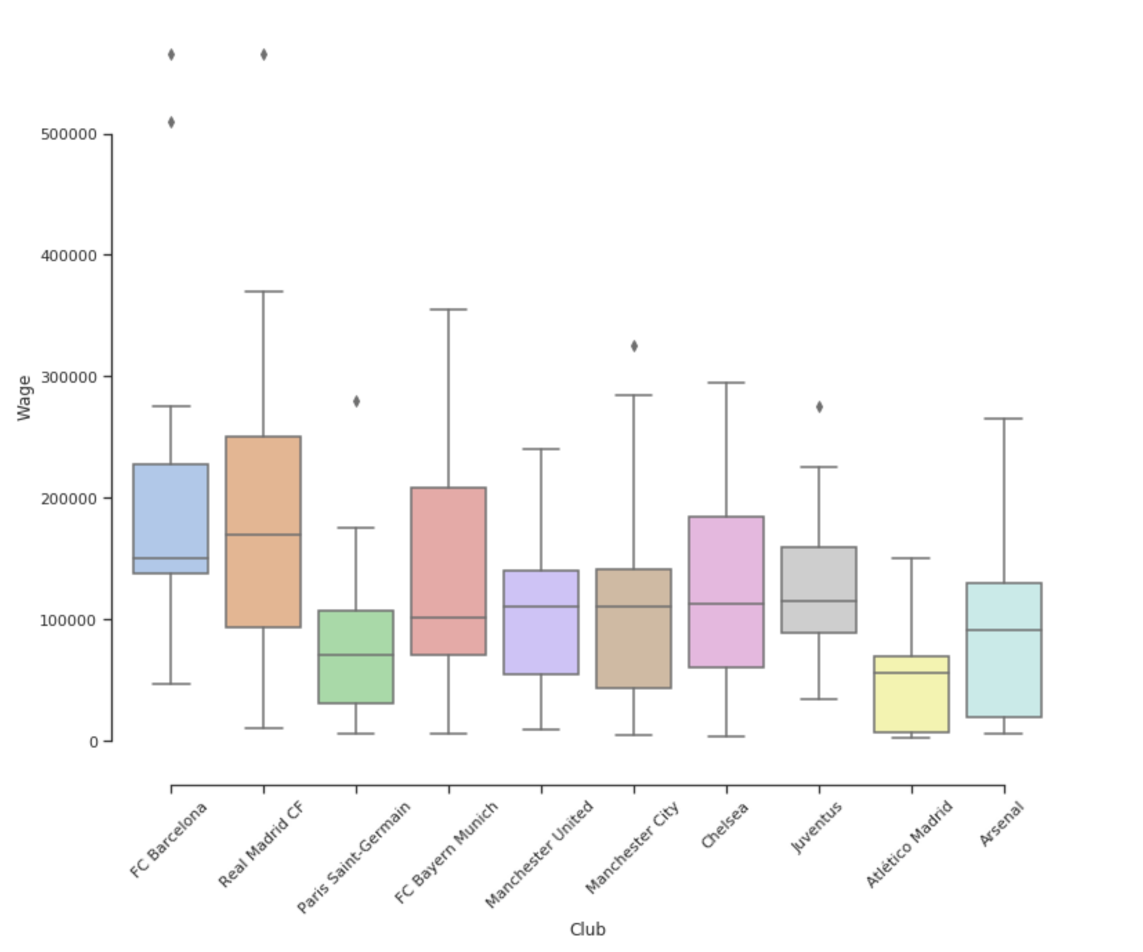
A quick way to understand which clubs command the highest salaries is to plot the wages as a box-plot. This gives all the important statistical metrics as well as the spread about the mean.To do this analysis, the top 10 clubs by median overall rating were chosen and their wages depicted as box plots.
| By Wage | By Player Value |
|---|---|
 |
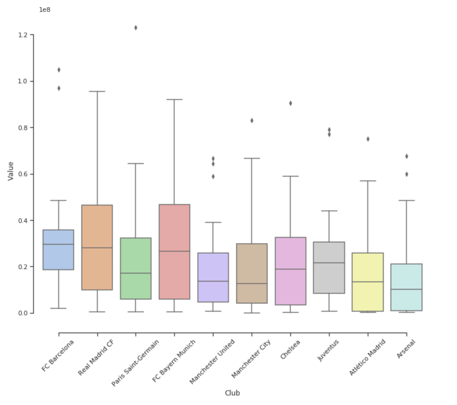 |
Real Madrid is seen to have the highest wage in terms of mean wage, followed by FC Barcelona and Manchester United and Manchester City. A real world application of this analysis can be used by players to decide which club they should strive for if they want a wage hike. Also in terms of most valuable players, Real Madrid and FC Bayern Munich seem to lead the pack.
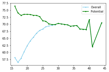
All players have been rated according to their overall performance as well as their potential rating in the future. On basic visual analysis of data it was noticed that a few of the older players had already reached their potential rating. To further delve into this and find an age where overall met the potential, the data was grouped by age and at each age, the average overall and average potential were calculated. These values were plotted as a line graph against the age as the line graph would show a clear trend of changes in these ratings and also if the ratings met at a certain point.
As we can see from the above graph, we notice that overall and potential meet approximately at around age 29 and continue to match as the age goes up. Another interesting tend that was observed is that while overall increases as age increases and peaks between the years 29 to 33, the potential rating actually decreases as age progresses till it meets the potential and then plateaus. There are very few players above the age of 37 and have been ignored as outliers. This analysis can be useful for while creating a squad as the age can be used as a factor in deciding whether a player should be retained or dropped. A way that this can be further enhanced is to find the trend of each player attribute across ages to determine the age at which each player attribute peaks.
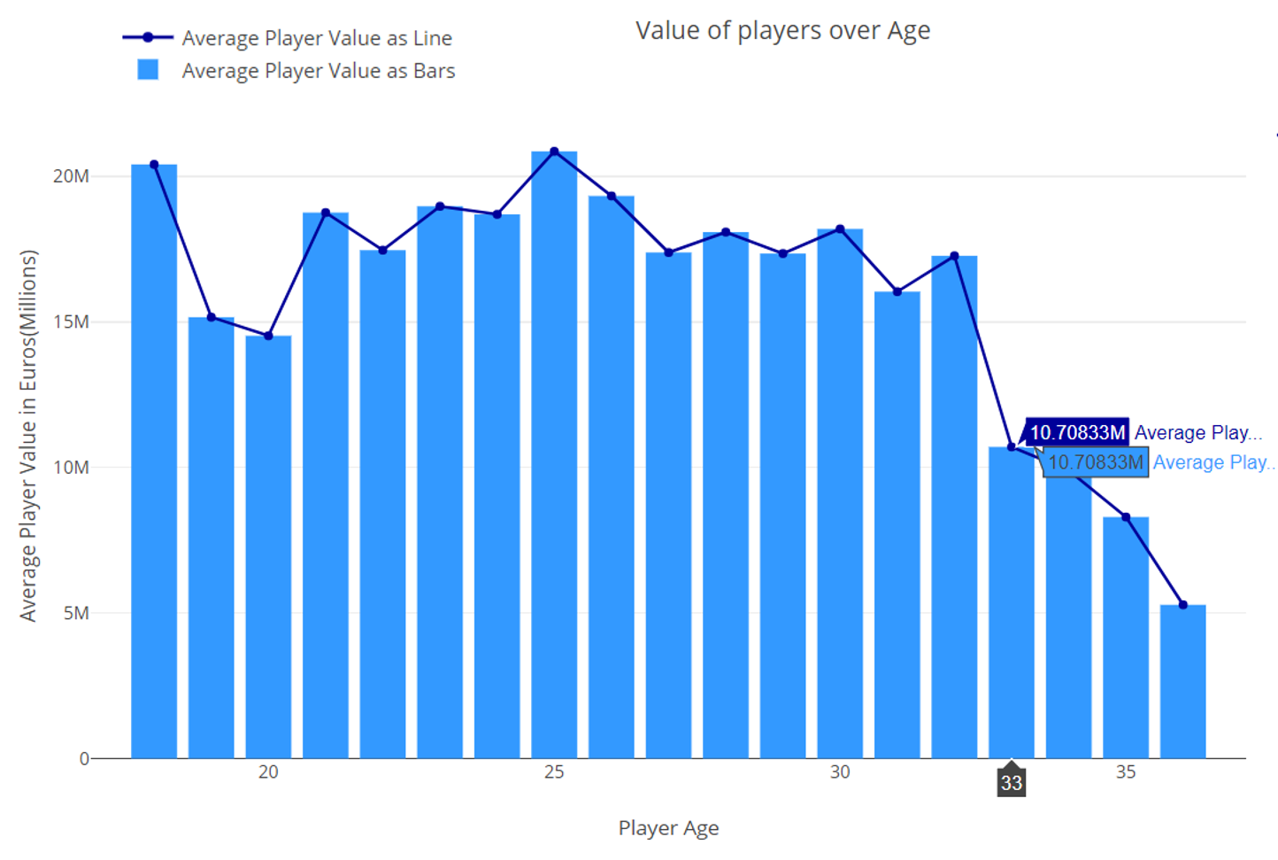
Here we will be analyzing the mean player value over ages 18 to 36, for the top 1000 players ranked as per their overall potential. We have used a bar chart along with a line chart here to display the data, with the ages on the x-axis and the average player value (in millions of Euros) on the y-axis. The observations from this chart can be used by both new players as well association football management to get an idea of current player valuation trends with regards to players at different ages.
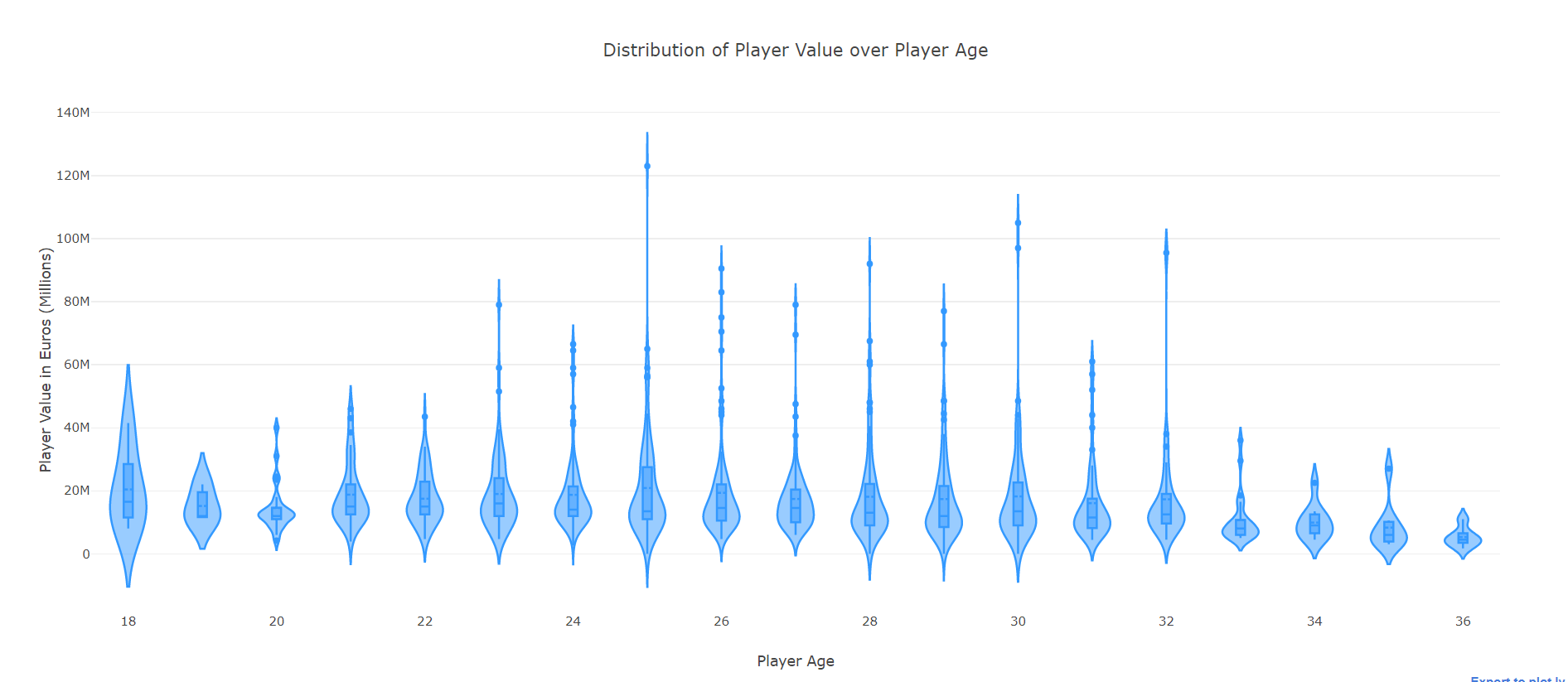
As per this chart, we can see that are two peaks for player value – One right at age 18(20.4 M Euros), and the other at age 25(20.8 M Euros). This seems to indicate that young players entering 18 years of age tend to be traded at high values across clubs due to their sheer potential. After 18, there appears to be a sharp drop at age 19. Average player value rises from age 19 onwards to peak at 25, following which there is gradual decline till age 32. Player value sharply falls after that, most likely due to the fact that older players in their mid-late 30s are considered to have spent their potential by then and have less resale value among clubs, in spite of the fact that they are more experienced. Next we have focused on the distribution of player value over the ages as opposed to previous plot of average values. For this purpose we have used violin plots, with box plot within. The violin plot is more informative than a simple box plot here because not only does it convey the distribution of the Player Value at each age (through Min,Q1,Median,Q3,Max) but it also shows the kernel density i.e. how common each player value point is by the width of its shape.
The observations here are that most player (between Q1 and Q3) across all ages have nearly violin width. It’s the high performing players who are outliers and pulling up average values at each age. One departure however is again at the age 18, where from the shape of the violin we can make out that 18 year old players are most evenly distributed in the range 8-36 Million. Thus players debuting at age 18 have confirmed chance of being valued highly. Also from the distribution it is apparent that player valuation decreases post 32 for nearly all players apparent from the violin density.
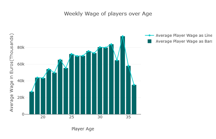
We have used box plots and line plots to show the average weekly wage of players (y-axis) versus the age of players (x-axis). As before we are only considering the subset of top 1000 players aged between 18 and 36. Like the valuation data, observations from this plot can be used by new players and association football management to get an idea of current player wages for different age groups.
Unlike with Player Value, Average Player weekly Wage is at its lowest(27K Euros) at 18 years age and then steadily rises till peaking(93.6K Euros) at age 34, and then from there it starts to fall. This trend shows us that whereas Player Value was more dependent on the potential of the player, player wages are more affected by the experience of the player and their seniority in teams.. The increase in player weekly wage is also much more gradual with age as compared to player value, which was prone to much variation. One anomaly is the sharp dip in average weekly wage at age 33 as compared to ages 32 and 34. This can be attributed to the fact that there may not be many players currently in the top 1000 who are of age 33, and the ones who are there seem to have lower weekly wage values.
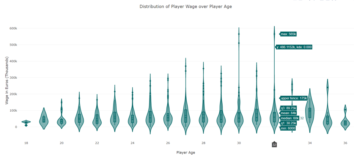
In the next plot we try to focus on the distribution of the weekly wage values versus age using violin plots (with box plots inset inside them). Again we use the violin plot here as it is much more informative in terms of showing probability of how much of the player population is occurring at a particular value of weekly wage for a particular age group.
Here we observe that almost across all ages the weekly wage is uniformly distributed 25-75k range as apparent from the distribution of density kernel shape. The average weekly wage is however being driven up due to extremely well paid players in each group, which are visible as outlying points in the point. From ages 25-32 we can also see that there is a large distribution of players who earn more than 100K euros a week. Not surprisingly almost all 18 year olds are clustered around the same starting weekly wage value, almost all distribution across the density kernel width is at around 30K. Players at age 34 seem to have the most uniform distribution of weekly wage, with nearly 75% in the middle have weekly wages in the range 60K to 115K.
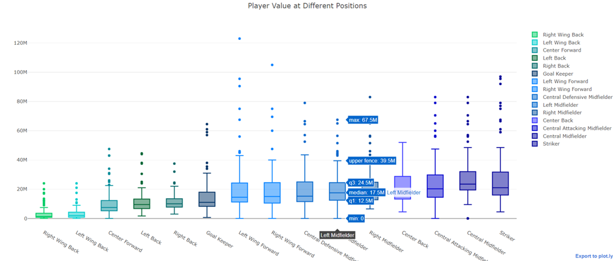
Here we attempt to show the distribution of player value at different positions. We have associated each player to their preferred position or where they are most likely to play (available in the data as an array of preferred positions for each player). We are making use of box plots with whiskers as well outliers to show the distribution of player value across all popularly played positions in football. Observations from the box plot can help new players and managers get an idea of current player valuation trends at each position.
From plotting the data one can see there are clear divisions in player valuation across player position. For the purpose of comparison we are only using the top 100 players in each position. The group with least valuation is of the two wing backs (right and left) having a median valuation of just 1.4-2.1M Euros. This is followed by a group consisting of 4 positions with nearly same valuations – Center Forward, Left Back, Right Back and the Goalkeeper. Surprisingly Center forward which used to be a traditional forward role seems to be eclipsed by roles such as Strikers and Central Attacking Midfielders. The median valuation for Center forwards is 7.5M. Left and Right back defenders have median values of 9.5-10M Euros and Goalkeepers round off this group with median player value of 11M. However there are a lot of goalkeeper outliers who have value of as much as around 60M.
The next group consists of the Left and Right wing forwards, Central Defensive midfielder, and the left and right midfielders. All these positions have a player value median in the range of 14.5M to 18.5M. Though players between Q1 and Q3 are almost evenly distributed across these groups, it’s the outliers here which are most distinctive. Neymar with a valuation of 123M is a distinct left forward outliers. Others include Lionel Messi at 105M as well as Christiano Ronaldo at 95.5M as right forwards. The next and most valued group consists of the Center Back, the Central Attacking Midfielder, Central Midfielder and finally the Striker. The median value varies from 19 to 23.5M for this group, with both midfielder and the striker positions having many high value outliers like Luis Suarez who as a striker is valued at 97M Euros.
In the FIFA 18 dataset, there is a score by each player for every possible position on the field. Some players are more versatile, and have good rankings for multiple positions as well. We have tried to get the top 10 players by their position score (not overall/potential) to make an informed choice of which player to pick for which position. The most appropriate way to show any data with only categorical (explanatory) variables, is not as a graph but a table. Hence, we have gone with a simple tabular representation where the rankings of the 10 players (in decreasing order of their potential to score) for each position has been shown.
L. Messi and C. Ronaldo seem to be the most consistent players of the lot having top rankings at over 3 positions. Some players have top rankings in a single position category making them the best but don’t appear anywhere in other categories like T.Kroos. As a general trend it is noticed that top players of each position play consistently across Center, left, and right positions of the same category.
This can be used to make smart & informed decisions about which player to pick for what position not just independently but relatively seeing rankings and consistency of choices across the board. This always gives a good idea of betting odds of a player to success when he is already playing at a certain position.
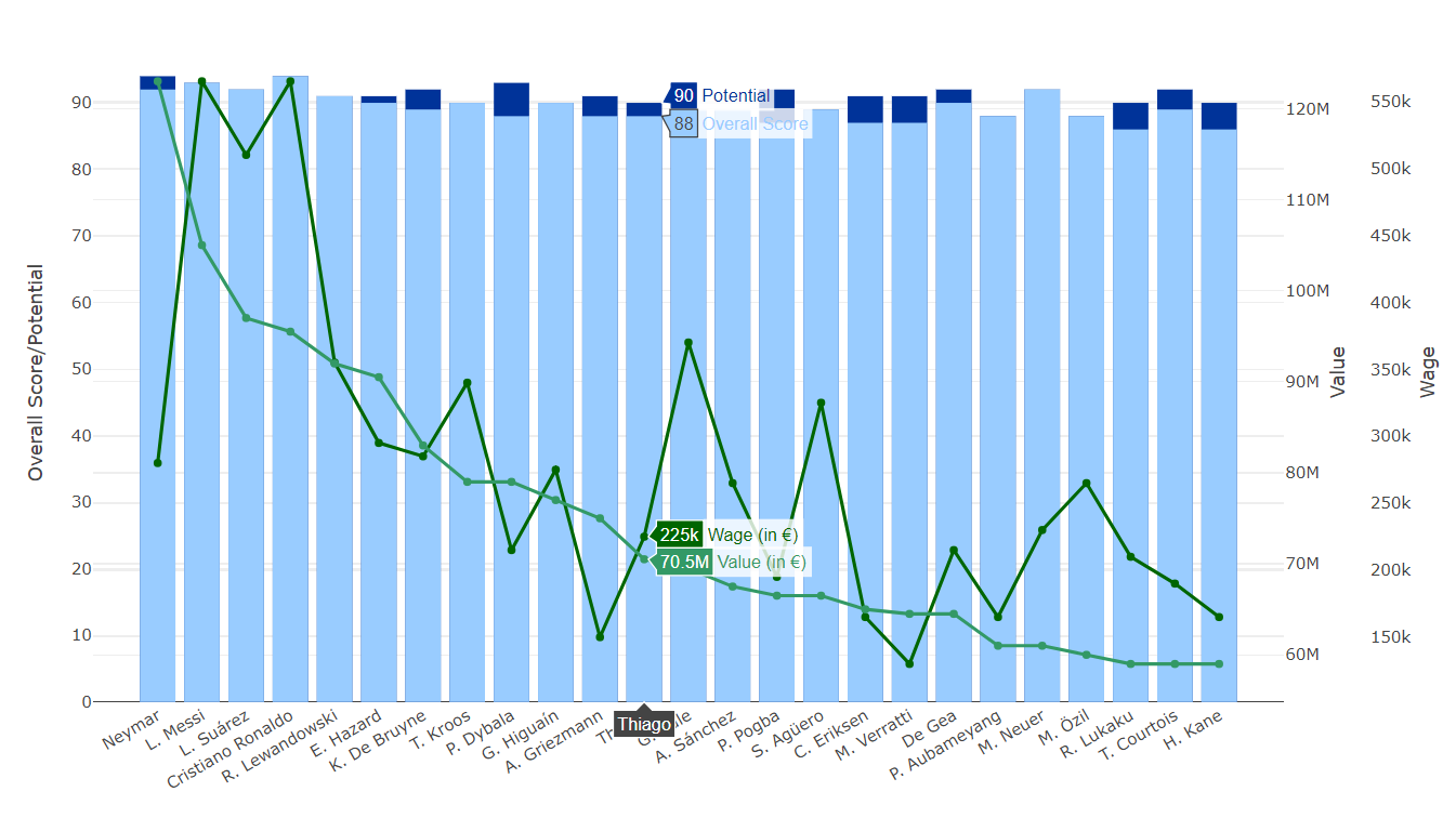
Players have two monetary attributes to them – Wage and Value. There is a large variation between the numbers both in terms of scale, delta difference, and consistency. We wanted to find out if the most valuable players are actually worth that much when to comes to wages. Also, we wanted to see if there is a common trend of players being value higher with comparison to their potential.We chose to present this using a multi axis chart combination chart because of different axis scales for `Overall Score + Potential (on primary y axis)`, `Value (secondary y axis)`, `Wage (Secondary 2 y axis)`. Stacked bar for `Score` and `Potential` because `Potential >= Overall` score so this will give us an idea of players performing to maximum potential and otherwise.
We found out that Neymar – the player with the highest value lies in the lower wage category of Top 25 most valued players whereas Sanchez and S. Aguero have wages in Top 5 despite being ranked in the lower side of most valued players. L. Messi, L. Suarez, and C. Ronaldo seem to be most consistent in both categories and have also performed to the best of their potential. P. Dybala and P. Pogba have the most difference between Potential and performance.
We discovered that wages and values do not necessarily correlate with each other in a direct sense, the next step of further improvement would be to find out the factors that affect the value and wage and wages of a player and their corresponding significance (coefficients).
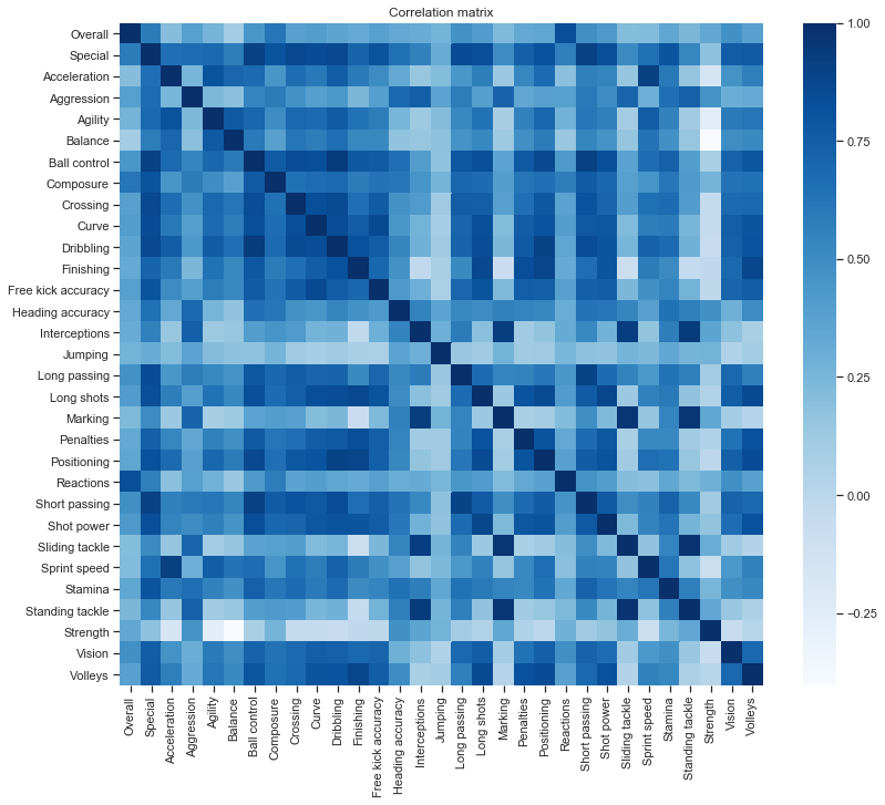
Speaking of player attributes, there are 35 skills across which all the players have been rated. These ratings contribute to the player’s overall rating and potential. An effort was made to understand which skills are highly correlated with the overall and potential ratings of players. To help perform and visualize the analysis, a correlation matrix was plotted and displayed as a heatmap. The heatmap, which its color-coded scale of correlation coefficient gives a quick overview of which skills are highly correlated and which are negatively correlated. The darker the color of the square, the more is the correlation.
To deduce which are the skills correlated with the overall, we chose a correlation coefficient greater than or equal to 0.5. Anything between 0.3 and 0.5 is attributed to being mildly correlated.
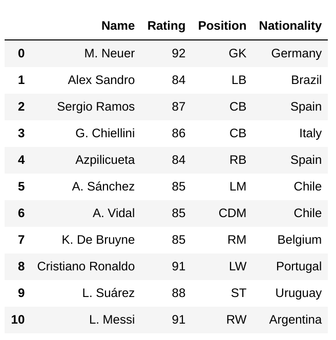
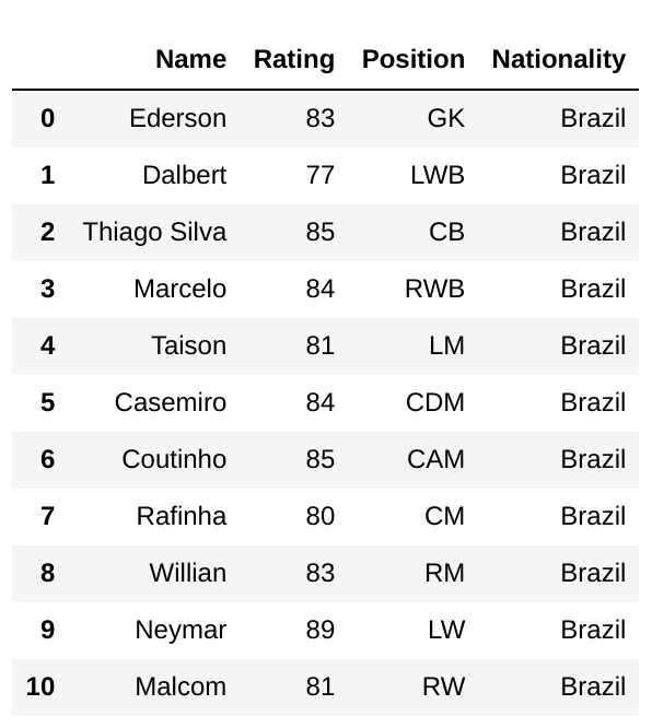
The aim in this section is to use statistical analysis on our data to find out the best squad for a dream team given a user selected formation, nationality and/or club. For every given playing formation the program computes the best players for each position in that formation and gives you the best possible player.
The program takes input for the following 3 parameters:
Formation (3-5-2, 4-4-2, 4-3-3, 3-4-3, 5-3-2) Nationality (and/or) Club
The best team for 4-3-3 formation predicted by the program was:
The best team for 3-5-2 formation for the country Brazil predicted by the program was:
The ultimate goal of our approach is to assign optimal position to the players depending on their skillset. In this case, three output classes are pre-decided: attack, mid and defense. Since there are many features that are not relevant to deduce our results, we can drop them. Thus, the selection of 30 relevant features is done for improving the accuracy of the model by supplying quality data to the classifier. For example, attributes like personal information are futile for training the classifier and thus can be ignored for analysis. The dataset has a column where the preferred position of the player is stated. A total of 14 positions are then mapped to the 3 predecided classes.
The machine learning models used in this approach are Random Forests and Logistic Regression. In case of Logistic Regression, Multinomial Logistic Regression is used since the dependent classes is a multi-class. Random forests is used with default parameters.
The top 10 most important features for the prediction were :
            Attributes                    Coef
0            Finishing     0.09187908935469322
1          Positioning     0.04294413649854606
2         Long passing    0.034394793890987395
3            Reactions     0.03356310980569168
4              Volleys     0.02922170807979512
5        Short passing    0.024554753581556697
6         Ball control    0.019851379649650565
7             Crossing     0.01869540014896692
8          GK reflexes    0.016953298324941423
9              Marking    0.016796213892711038
10 Sprint speed 0.01670935869115817LIBRARIES
- numpy
- pandas
- plotly
- seaborn
- json
- matplotlib
- itertools
- sklearn
- IPython
- string
- re
WEBSITES
- https://stackoverflow.com/
- https://kaggle.com/
- https://seaborn.pydata.org/
- https://seaborn.pydata.org/examples/index.html
- https://wiki.python.org/moin/PythonGraphLibraries
- https://python-graph-gallery.com/
- https://github.com/
- https://plot.ly/python/
- https://pandas.pydata.org/
Changes and Improvement suggestions are welcome. Feel free to comment new additions that you think are useful or drop a PR on the github project.
Wanna buy me coffee - paypal.me/AShrivastava961
