scikit-mobility is a library for human mobility analysis in Python. The library allows to:
-
represent trajectories and mobility flows with proper data structures,
TrajDataFrameandFlowDataFrame. -
manage and manipulate mobility data of various formats (call detail records, GPS data, data from Location Based Social Networks, survey data, etc.);
-
extract human mobility metrics and patterns from data, both at individual and collective level (e.g., length of displacements, characteristic distance, origin-destination matrix, etc.)
-
generate synthetic individual trajectories using standard mathematical models (random walk models, exploration and preferential return model, etc.)
-
generate synthetic mobility flows using standard migration models (gravity model, radiation model, etc.)
-
assess the privacy risk associated with a mobility dataset
https://scikit-mobility.github.io/scikit-mobility/
if you use scikit-mobility please cite the following paper: https://arxiv.org/abs/1907.07062
@misc{pappalardo2019scikitmobility,
    title={scikit-mobility: a Python library for the analysis, generation and risk assessment of mobility data},
    author={Luca Pappalardo and Filippo Simini and Gianni Barlacchi and Roberto Pellungrini},
    year={2019},
    eprint={1907.07062},
    archivePrefix={arXiv},
    primaryClass={physics.soc-ph}
}
First, clone the repository - this creates a new directory ./scikit_mobility.
git clone https://github.com/scikit-mobility/scikit-mobility scikit_mobility
-
Create an environment
skmoband install pipconda create -n skmob pip python=3.7 -
Activate
source activate skmob -
Install skmob
 cd scikit_mobility
 python setup.py install
If the installation of a required library fails, reinstall it with
conda install. -
OPTIONAL to use
scikit-mobilityon the jupyter notebook-
Install the kernel
conda install ipykernel -
Open a notebook and check if the kernel
skmobis on the kernel list. If not, run the following:env=$(basename `echo $CONDA_PREFIX`) python -m ipykernel install --user --name "$env" --display-name "Python [conda env:"$env"]"
-
❗ You may run into dependency issues if you try to import the package in Python. If so, try installing the following packages as followed.
conda install -n skmob pyproj urllib3 chardet markupsafe
-
Create an environment
skmobpython3 -m venv skmob -
Activate
source skmob/bin/activate -
Install skmob
cd scikit_mobility python setup.py install -
OPTIONAL to use
scikit-mobilityon the jupyter notebook-
Activate the virutalenv:
source skmob/bin/activate -
Install jupyter notebook:
pip install jupyter -
Run jupyter notebook
jupyter notebook -
(Optional) install the kernel with a specific name
ipython kernel install --user --name=skmob
-
> source activate skmob
(skmob)> python
>>> import skmob
>>>
In scikit-mobility, a set of trajectories is described by a TrajDataFrame, an extension of the pandas DataFrame that has specific columns names and data types. A row in the TrajDataFrame represents a point of the trajectory, described by three mandatory fields (aka columns):
latitude(type: float);longitude(type: float);datetime(type: date-time).
Additionally, two optional columns can be specified:
uid(type: string) identifies the object associated with the point of the trajectory. Ifuidis not present, scikit-mobility assumes that theTrajDataFramecontains trajectories associated with a single moving object;tidspecifies the identifier of the trajectory to whichthe point belongs to. Similar touid, iftidis not present, scikit-mobility assumes that theTrajDataFramecontains a single trajectory;
Note that, besides the mandatory columns, the user can add to a TrajDataFrame as many columns as they want since the data structures in scikit-mobility inherit all the pandas DataFrame functionalities.
Create a TrajDataFrame from a list:
>>> import skmob
>>> # create a TrajDataFrame from a list
>>> data_list = [[1, 39.984094, 116.319236, '2008-10-23 13:53:05'], [1, 39.984198, 116.319322, '2008-10-23 13:53:06'], [1, 39.984224, 116.319402, '2008-10-23 13:53:11'], [1, 39.984211, 116.319389, '2008-10-23 13:53:16']]
>>> tdf = skmob.TrajDataFrame(data_list, latitude=1, longitude=2, datetime=3)
>>> print(tdf.head())
   0        lat         lng            datetime
0  1  39.984094  116.319236 2008-10-23 13:53:05
1  1  39.984198  116.319322 2008-10-23 13:53:06
2  1  39.984224  116.319402 2008-10-23 13:53:11
3  1  39.984211  116.319389 2008-10-23 13:53:16
>>> print(type(tdf))
<class 'skmob.core.trajectorydataframe.TrajDataFrame'>
Create a TrajDataFrame from a pandas DataFrame:
>>> import pandas as pd
>>> # create a DataFrame from the previous list
>>> data_df = pd.DataFrame(data_list, columns=['user', 'latitude', 'lng', 'hour'])
>>> print(type(data_df))
<class 'pandas.core.frame.DataFrame'>
>>> # now create a TrajDataFrame from the pandas DataFrame
>>> tdf = skmob.TrajDataFrame(data_df, latitude='latitude', datetime='hour', user_id='user')
>>> print(type(tdf))
<class 'skmob.core.trajectorydataframe.TrajDataFrame'>
>>> print(tdf.head())
   uid        lat         lng            datetime
0    1  39.984094  116.319236 2008-10-23 13:53:05
1    1  39.984198  116.319322 2008-10-23 13:53:06
2    1  39.984224  116.319402 2008-10-23 13:53:11
3    1  39.984211  116.319389 2008-10-23 13:53:16
Create a TrajDataFrame from a file:
>>> # download the file from https://raw.githubusercontent.com/scikit-mobility/scikit-mobility/master/tutorial/data/geolife_sample.txt.gz
>>> # read the trajectory data (GeoLife, Beijing, China)
>>> tdf = skmob.TrajDataFrame.from_file('geolife_sample.txt.gz', latitude='lat', longitude='lon', user_id='user', datetime='datetime')
>>> print(tdf.head())
	 lat         lng            datetime  uid
0  39.984094  116.319236 2008-10-23 05:53:05    1
1  39.984198  116.319322 2008-10-23 05:53:06    1
2  39.984224  116.319402 2008-10-23 05:53:11    1
3  39.984211  116.319389 2008-10-23 05:53:16    1
4  39.984217  116.319422 2008-10-23 05:53:21    1
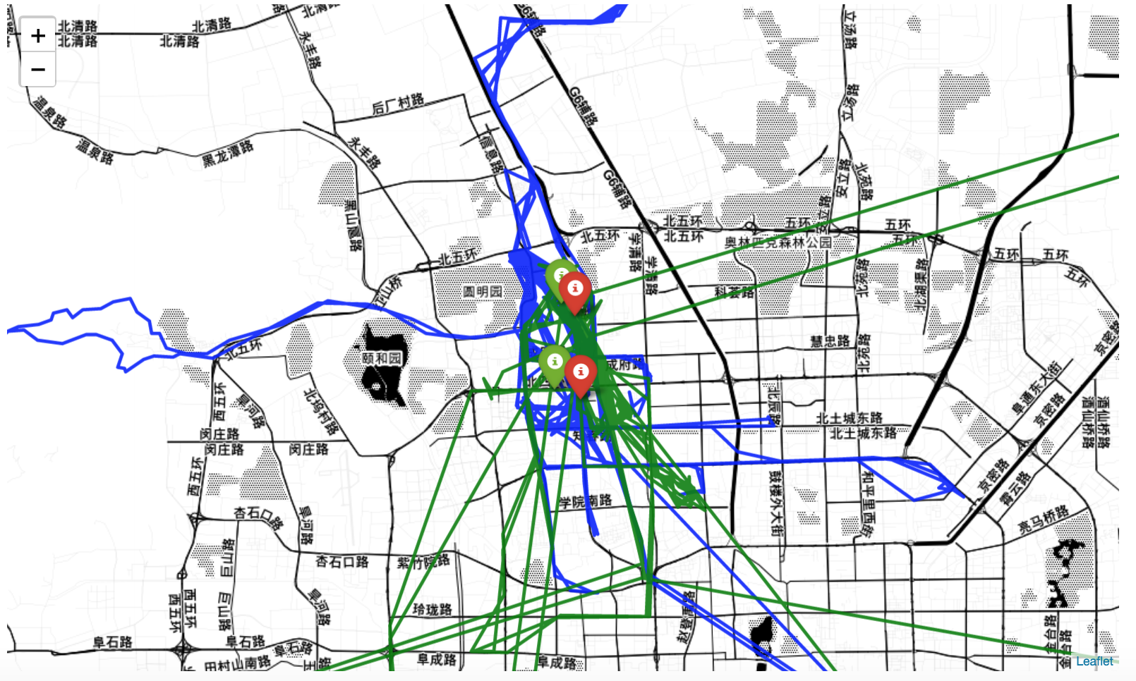
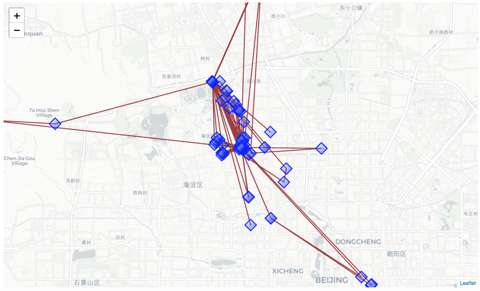
A TrajDataFrame can be plotted on an folium interactive map using the plot_trajectory function.
>>> tdf.plot_trajectory(zoom=12, weight=3, opacity=0.9, tiles='Stamen Toner')
In scikit-mobility, an origin-destination matrix is described by the FlowDataFrame structure, an extension of the pandas DataFrame that has specific column names and data types. A row in a FlowDataFrame represents a flow of objects between two locations, described by three mandatory columns:
origin(type: string);destination(type: string);flow(type: integer).
Again, the user can add to a FlowDataFrame as many columnsas they want. Each FlowDataFrame is associated with a spatial tessellation, a geopandas GeoDataFrame that contains two mandatory columns:
tile_ID(type: integer) indicates the identifier of a location;geometryindicates the polygon (or point) that describes the geometric shape of the location on a territory (e.g., a square, a voronoi shape, the shape of a neighborhood).
Note that each location identifier in the origin and destination columns of a FlowDataFrame must be present in the associated spatial tessellation.
Create a spatial tessellation from a file:
>>> import skmob
>>> import geopandas as gpd
>>> # load a spatial tessellation
>>> url_tess = 'https://raw.githubusercontent.com/scikit-mobility/scikit-mobility/master/tutorial/data/NY_counties_2011.geojson'
>>> tessellation = gpd.read_file(url_tess).rename(columns={'tile_id': 'tile_ID'})
>>> print(tessellation.head())
  tile_ID  population                                           geometry
0   36019       81716  POLYGON ((-74.006668 44.886017, -74.027389 44....
1   36101       99145  POLYGON ((-77.099754 42.274215, -77.0996569999...
2   36107       50872  POLYGON ((-76.25014899999999 42.296676, -76.24...
3   36059     1346176  POLYGON ((-73.707662 40.727831, -73.700272 40....
4   36011       79693  POLYGON ((-76.279067 42.785866, -76.2753479999...
Create a FlowDataFrame from a spatial tessellation and a file of flows:
>>> # load real flows into a FlowDataFrame
>>> # download the file with the real fluxes from: https://raw.githubusercontent.com/scikit-mobility/scikit-mobility/master/tutorial/data/NY_commuting_flows_2011.csv
>>> fdf = skmob.FlowDataFrame.from_file("NY_commuting_flows_2011.csv",
                                    tessellation=tessellation,
                                    tile_id='tile_ID',
                                    sep=",")
>>> print(fdf.head())
     flow origin destination
0  121606  36001       36001
1       5  36001       36005
2      29  36001       36007
3      11  36001       36017
4      30  36001       36019
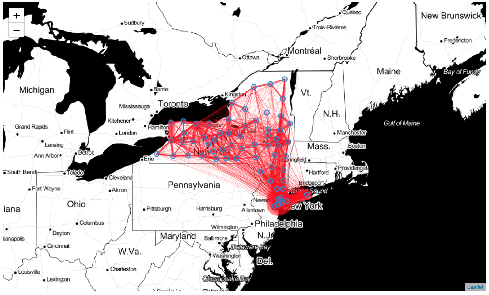
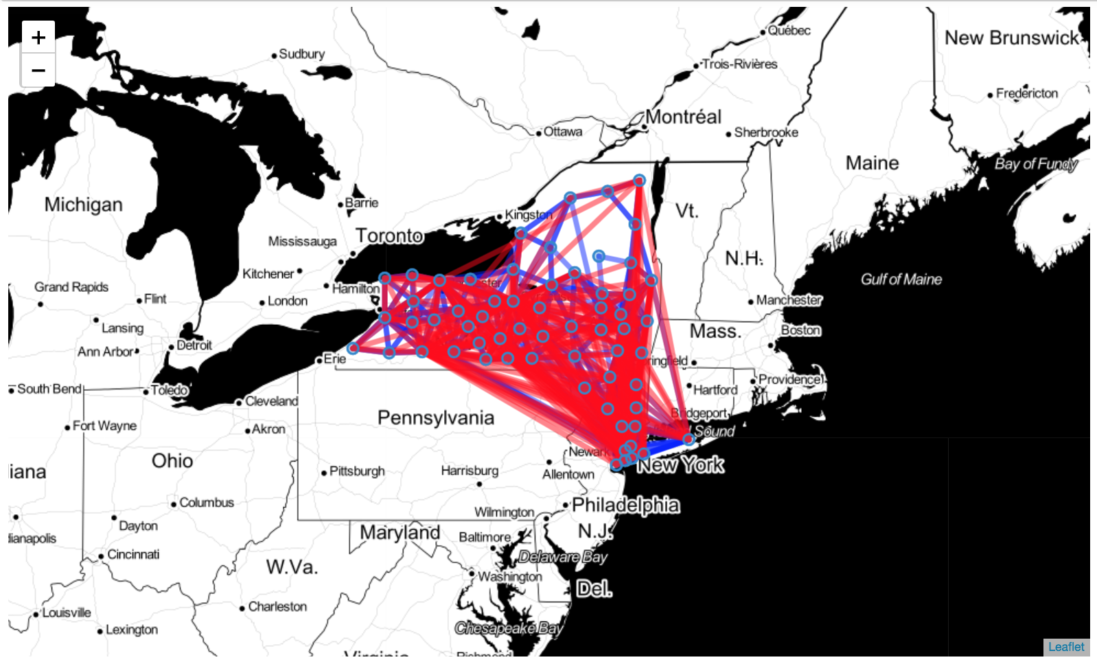
A FlowDataFrame can be visualized on a folium interactive map using the plot_flows function, which plots the flows on a geographic map as lines between the centroids of the tiles in the FlowDataFrame's spatial tessellation:
>>> fdf.plot_flows(flow_color='red')
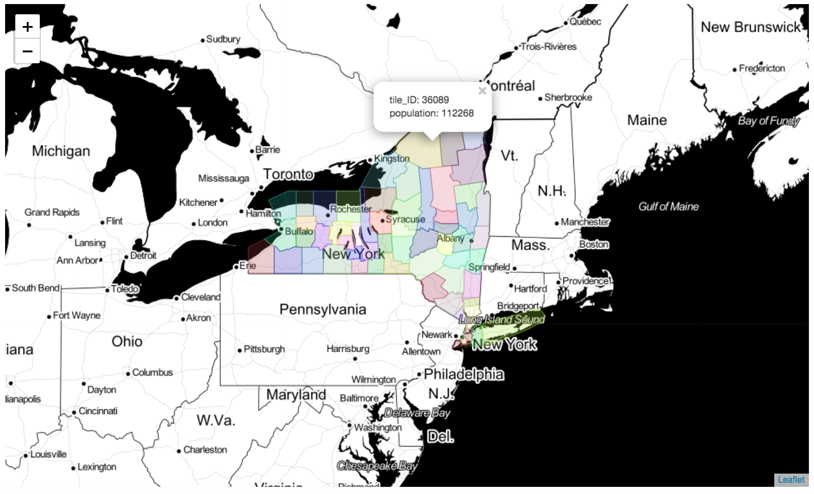
Similarly, the spatial tessellation of a FlowDataFrame can be visualized using the plot_tessellation function. The argument popup_features (type:list, default:[constants.TILE_ID]) allows to enhance the plot's interactivity displaying popup windows that appear when the user clicks on a tile and includes information contained in the columns of the tessellation's GeoDataFrame specified in the argument’s list:
>>> fdf.plot_tessellation(popup_features=['tile_ID', 'population'])
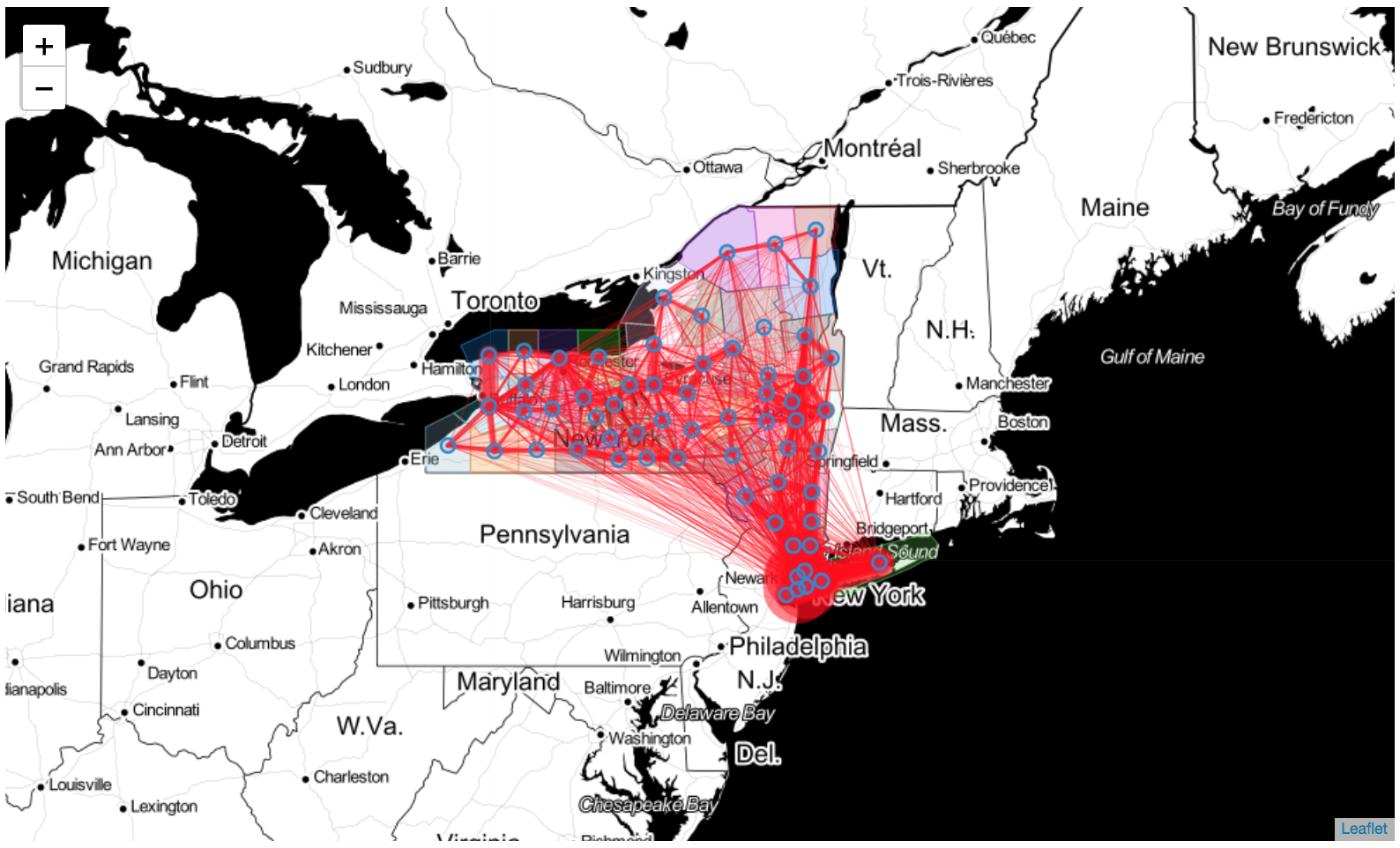
The spatial tessellation and the flows can be visualized together using the map_f argument, which specified the folium object on which to plot:
>>> m = fdf.plot_tessellation()
>>> fdf.plot_flows(flow_color='red', map_f=m)
As any analytical process, mobility data analysis requires data cleaning and preprocessing steps. The preprocessing module allows the user to perform four main preprocessing steps:
- noise filtering;
- stop detection;
- stop clustering;
- trajectory compression;
Note that, if TrajDataFrame contains multiple trajectories from multiple users, the preprocessing methods automatically apply to the single trajectory and, when necessary, to the single object.
In scikit-mobility, the standard method filter filters out a point if the speed from the previous point is higher than the parameter max_speed, whichis by default set to 500km/h.
>>> n_deleted_points = len(tdf) - len(ftdf) # number of deleted points
>>> print(n_deleted_points)
{'from_file': 'geolife_sample.txt.gz', 'filter': {'function': 'filter', 'max_speed_kmh': 500.0, 'include_loops': False, 'speed_kmh': 5.0, 'max_loop': 6, 'ratio_max': 0.25}}
>>> n_deleted_points = len(tdf) - len(ftdf) # number of deleted points
>>> print(n_deleted_points)
54
Note that the TrajDataFrame structure as the parameters attribute, which indicates the list of operations that have been applied to the TrajDataFrame. This attribute is a dictionary the key of which is the signature of the function applied.
Some points in a trajectory can represent Point-Of-Interests (POIs) such as schools, restaurants, and bars, or they can represent user-specific places such as home and work locations. These points are usually called Stay Points or Stops, and they can be detected in different ways. A common approach is to apply spatial clustering algorithms to cluster trajectory points by looking at their spatial proximity. In scikit-mobility, the stops function, contained in the detection module, finds the stay points visited by an object. For instance, to identify the stops where the object spent at least minutes_for_a_stop minutes within a distance spatial_radius_km \time stop_radius_factor, from a given point, we can use the following code:
>>> from skmob.preprocessing import detection
>>> stdf = detection.stops(tdf, stop_radius_factor=0.5, minutes_for_a_stop=20.0, spatial_radius_km=0.2, leaving_time=True)
>>> print(stdf.head())
	 lat         lng            datetime  uid    leaving_datetime
0  39.978030  116.327481 2008-10-23 06:01:37    1 2008-10-23 10:32:53
1  40.013820  116.306532 2008-10-23 11:10:19    1 2008-10-23 23:45:27
2  39.978419  116.326870 2008-10-24 00:21:52    1 2008-10-24 01:47:30
3  39.981166  116.308475 2008-10-24 02:02:31    1 2008-10-24 02:30:29
4  39.981431  116.309902 2008-10-24 02:30:29    1 2008-10-24 03:16:35
>>> print('Points of the original trajectory:\t%s'%len(tdf))
>>> print('Points of stops:\t\t\t%s'%len(stdf))
Points of the original trajectory:	217653
Points of stops:			391
A new column leaving_datetime is added to the TrajDataFrame in order to indicate the time when the user left the stop location. We can then visualize the detected stops using the plot_stops function:
>>> m = stdf.plot_trajectory(max_users=1, start_end_markers=False)
>>> stdf.plot_stops(max_users=1, map_f=m)
The goal of trajectory compression is to reduce the number of trajectory points while preserving the structure of the trajectory. This step results in a significant reduction of the number of trajectory points. In scikit-mobility, we can use one of the methods in the compression module under the preprocessing module. For instance, to merge all the points that are closer than 0.2km from each other, we can use the following code:
>>> from skmob.preprocessing import compression
>>> # compress the trajectory using a spatial radius of 0.2 km
>>> ctdf = compression.compress(tdf, spatial_radius_km=0.2)
>>> print('Points of the original trajectory:\t%s'%len(tdf))
>>> print('Points of the compressed trajectory:\t%s'%len(ctdf))
Points of the original trajectory:	217653
Points of the compressed trajectory:	6281
Several measures have been proposed in the literature to capture the patterns of human mobility, both at the individual and collective levels. Individual measures summarize the mobility patterns of a single moving object, while collective measures summarize mobility patterns of a population as a whole. scikit-mobility provides a wide set of mobility measures, each implemented as a function that takes in input a TrajDataFrame and outputs a pandas DataFrame. Individual and collective measures are implemented the in skmob.measure.individual and the skmob.measures.collective modules, respectively.
For example, the following code compute the radius of gyration, the jump lengths and the home locations of a TrajDataFrame:
>>> from skmob.measures.individual import jump_lengths, radius_of_gyration, home_location
>>> # load a TrajDataFrame from an URL
>>> url = "https://snap.stanford.edu/data/loc-brightkite_totalCheckins.txt.gz"
>>> df = pd.read_csv(url, sep='\t', header=0, nrows=100000,
         names=['user', 'check-in_time', 'latitude', 'longitude', 'location id'])
>>> tdf = skmob.TrajDataFrame(df, latitude='latitude', longitude='longitude', datetime='check-in_time', user_id='user')
>>> rg_df = radius_of_gyration(tdf)
>>> print(rg_df)
   uid  radius_of_gyration
0    0         1564.436792
1    1         2467.773523
2    2         1439.649774
3    3         1752.604191
4    4         5380.503250
>>> jl_df = jump_lengths(tdf.sort_values(by='datetime'))
>>> print(jl_df.head())
   uid                                       jump_lengths
0    0  [19.640467328877936, 0.0, 0.0, 1.7434311010381...
1    1  [6.505330424378251, 46.75436600375988, 53.9284...
2    2  [0.0, 0.0, 0.0, 0.0, 3.6410097195943507, 0.0, ...
3    3  [3861.2706300798827, 4.061631313492122, 5.9163...
4    4  [15511.92758595804, 0.0, 15511.92758595804, 1....
Note that for some measures, such as jump_length, the TrajDataFrame must be order in increasing order by the column datetime (see the documentation for the measures that requires this condition https://scikit-mobility.github.io/scikit-mobility/reference/measures.html).
>>> hl_df = home_location(tdf)
>>> print(hl_df.head())
   uid        lat         lng
0    0  39.891077 -105.068532
1    1  37.630490 -122.411084
2    2  39.739154 -104.984703
3    3  37.748170 -122.459192
4    4  60.180171   24.949728
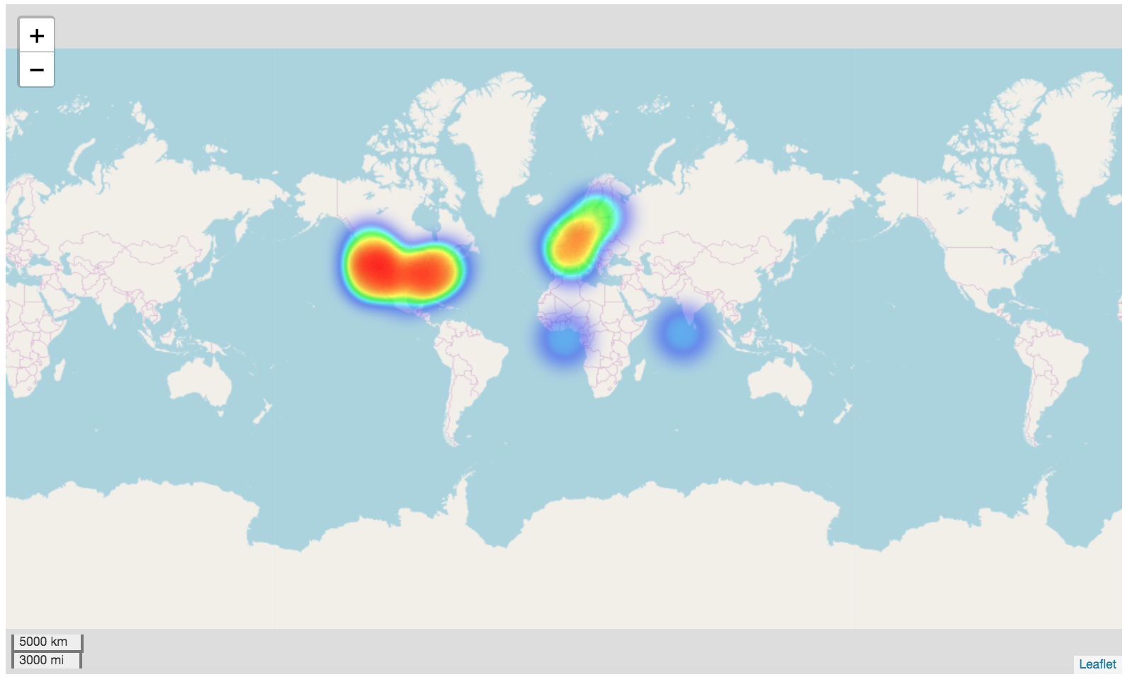
>>> # now let's visualize a cloropleth map of the home locations
>>> import folium
>>> from folium.plugins import HeatMap
>>> m = folium.Map(tiles = 'openstreetmap', zoom_start=12, control_scale=True)
>>> HeatMap(hl_df[['lat', 'lng']].values).add_to(m)
>>> m
Collective generative algorithms estimate spatial flows between a set of discrete locations. Examples of spatial flows estimated with collective generative algorithms include commut-ing trips between neighborhoods, migration flows between municipalities, freight shipmentsbetween states, and phone calls between regions.
In scikit-mobility, a collective generative algorithm takes in input a spatial tessellation, i.e., a geopandas GeoDataFrame. To be a valid input for a collective algorithm, the spatial tessellation should contain two columns, geometry and relevance, which are necessary to compute the two variables used by collective algorithms: the distance between tiles and the importance (aka "attractiveness") of each tile. A collective algorithm produces a FlowDataFrame that contains the generated flows and the spatial tessellation. scikit-mobility implements the most common collective generative algorithms:
- the
Gravitymodel; - the
Radiationmodel.
The class Gravity, implementing the Gravity model, has two main methods:
fit, which calibrates the model's parameters using aFlowDataFrame;generate, which generates the flows on a given spatial tessellation.
Load the spatial tessellation and a data set of real flows in a FlowDataFrame:
>>> from skmob.utils import utils, constants
>>> import geopandas as gpd
>>> from skmob.models import Gravity
>>> import numpy as np
>>> # load a spatial tessellation
>>> url_tess = 'https://raw.githubusercontent.com/scikit-mobility/scikit-mobility/master/tutorial/data/NY_counties_2011.geojson'
>>> tessellation = gpd.read_file(url_tess).rename(columns={'tile_id': 'tile_ID'})
>>> # download the file with the real fluxes from: https://raw.githubusercontent.com/scikit-mobility/scikit-mobility/master/tutorial/data/NY_commuting_flows_2011.csv
>>> fdf = skmob.FlowDataFrame.from_file("NY_commuting_flows_2011.csv",
					tessellation=tessellation,
					tile_id='tile_ID',
					sep=",")
>>> # compute the total outflows from each location of the tessellation (excluding self loops)
>>> tot_outflows = fdf[fdf['origin'] != fdf['destination']].groupby(by='origin', axis=0)['flow'].sum().fillna(0).values
>>> tessellation[constants.TOT_OUTFLOW] = tot_outflows
Instantiate a Gravity model object and generate synthetic flows:
# instantiate a singly constrained Gravity model
>>> gravity_singly = Gravity(gravity_type='singly constrained')
>>> print(gravity_singly)
Gravity(name="Gravity model", deterrence_func_type="power_law", deterrence_func_args=[-2.0], origin_exp=1.0, destination_exp=1.0, gravity_type="singly constrained")
>>> # generate the synthetic flows
>>> np.random.seed(0)
>>> synth_fdf = gravity_singly.generate(tessellation,
				   tile_id_column='tile_ID',
				   tot_outflows_column='tot_outflow',
				   relevance_column= 'population',
				   out_format='flows')
>>> print(synth_fdf.head())
  origin destination  flow
0  36019       36101   101
1  36019       36107    66
2  36019       36059  1041
3  36019       36011   151
4  36019       36123    33
Fit the parameters of the Gravity model from the FlowDataFrame and generate the synthetic flows:
>>> # fit the parameters of the Gravity model from real fluxes
>>> gravity_singly_fitted = Gravity(gravity_type='singly constrained')
>>> print(gravity_singly_fitted)
>>> # fit the parameters of the Gravity from the FlowDataFrame
>>> gravity_singly_fitted.fit(fdf, relevance_column='population')
>>> print(gravity_singly_fitted)
Gravity(name="Gravity model", deterrence_func_type="power_law", deterrence_func_args=[-1.9947152031914186], origin_exp=1.0, destination_exp=0.6471759552223144, gravity_type="singly constrained")
>>> # generate the synthetics flows
>>> np.random.seed(0)
>>> synth_fdf_fitted = gravity_singly_fitted.generate(tessellation,
							tile_id_column='tile_ID',
							tot_outflows_column='tot_outflow',
							relevance_column= 'population',
							out_format='flows')
>>> print(synth_fdf_fitted.head())
  origin destination  flow
0  36019       36101   102
1  36019       36107    66
2  36019       36059  1044
3  36019       36011   152
4  36019       36123    33
Plot the real flows and the synthetic flows:
>>> m = fdf.plot_flows(min_flow=100, flow_exp=0.01, flow_color='blue')
>>> synth_fdf_fitted.plot_flows(min_flow=1000, flow_exp=0.01, map_f=m)
The Radiation model is parameter-free and has only one method: generate. Given a spatial tessellation, the synthetic flows can be generated using the Radiation class as follows:
>>> from skmob.models import Radiation
>>> np.random.seed(0)
>>> radiation = Radiation()
>>> rad_flows = radiation.generate(tessellation,
				tile_id_column='tile_ID',
				tot_outflows_column='tot_outflow',
				relevance_column='population',
				out_format='flows_sample')
>>> print(rad_flows.head())
  origin destination   flow
0  36019       36033  11648
1  36019       36031   4232
2  36019       36089   5598
3  36019       36113   1596
4  36019       36041    117
