Balanced Cut Tree Method for Hierarchical Clustering
This repo contains a small Python function that performs a balanced cut tree of a SciPy linkage matrix built using any linkage method (e.g. 'ward'). It builds upon the SciPy and NumPy libraries.
The initial problem was the following: if you perform a standard cut on a tree (i.e. the result from a hierarchical clustering), probably you will end up having a few big clusters (where the number of data samples is high), and many small clusters (each containing very few data samples). Thus, the resulting clustering is unbalanced, i.e. it contains clusters of very variable size.
The proposed function looks recursively along the hierarchical tree, from the root (single cluster gathering all the samples) to the leaves (i.e. the clusters with only one sample), retrieving the biggest possible clusters containing a number of samples lower than a given maximum. In this way, if a cluster at a specific tree level contains a number of samples higher than the given maximum, it is ignored and its offspring (smaller) sub-clusters are taken into consideration. If the cluster contains a number of samples lower than the given maximum, it is taken as result and its offspring sub-clusters not further processed.
Since all output clusters contain no more than a given maximum number of samples, the resulting clustering is considered to be more balanced than a standard tree cut. Note however that the number of samples per cluster might still have a considerable variability, since the splitting of a big cluster can result in sub-clusters with very variable number of samples. This variability should be smaller as the given maximum of samples per cluster is closer to 1 (being the variability equal to 0 when the maximum is at its limit, i.e. 1).
The function returns two results:
- List of integers containing for each input sample its corresponding cluster id. The cluster id is an integer which is higher for deeper tree levels.
- List of integer arrays containing for each input sample its corresponding cluster tree level, i.e. a sequence of 0s and 1s. Note that the cluster level is longer for deeper tree levels, being [0] the root cluster, [0, 0] and [0, 1] its offspring, and so on. Also note that in each cluster splitting, the label 0 denotes the bigger cluster, while the label 1 denotes the smallest.
Dependencies and Example Script
Before running the example script, please ensure you have installed the scipy and numpy packages in your Python environment.
In order to run the example script you can use the following command.
$ python3 cut_tree_balanced.py
By running the example script you should run commands and get printed outputs similar to the following.
First, a numpy array of 100 rows x 4 columns is randomly generated using a gamma distribution. Note that we perform such a random sampling from a gamma distribution so that the resulting standard clustering is unbalanced (see below). Similar results are obtained when varying the random seed.
    np.random.seed(4)
    X = gamma.rvs(0.1, size=400).reshape((100,4))
In order to check the validity of the input data, the type, shape and the first 10 rows are printed.
Type of the input data sample: <class 'numpy.ndarray'>
Shape of the input data sample: (100, 4)
First 10 rows of the input data:
[[1.28573793e-03 8.12672961e-06 1.26520704e-03 2.07729574e-03]
 [1.16397414e-01 2.06534197e-03 1.91044478e-02 5.35127859e-01]
 [5.81563428e-02 5.92302950e-06 1.90433024e-02 2.87155777e-02]
 [3.98932109e-08 5.37862343e-02 4.38562255e-02 1.27557329e-04]
 [3.57028885e-04 2.88945299e-05 3.40388733e-05 9.90278888e-06]
 [3.91282036e-06 4.61803593e-02 2.75652111e-08 1.66504104e-09]
 [2.60630428e-10 3.89770028e-04 8.52159994e-03 5.83321506e-09]
 [6.37325763e-10 3.41859809e-04 4.51815091e-02 2.83600476e-06]
 [1.14654357e-03 1.12808821e-02 1.61202749e-04 1.56459197e-11]]
Next, the linkage matrix is computed by using the ward method, and a standard tree cut is performed (with a specific number of output clusters = 20).
    Z = ward(X)
    standard_cut_cluster_id = cut_tree(Z, n_clusters=[20])
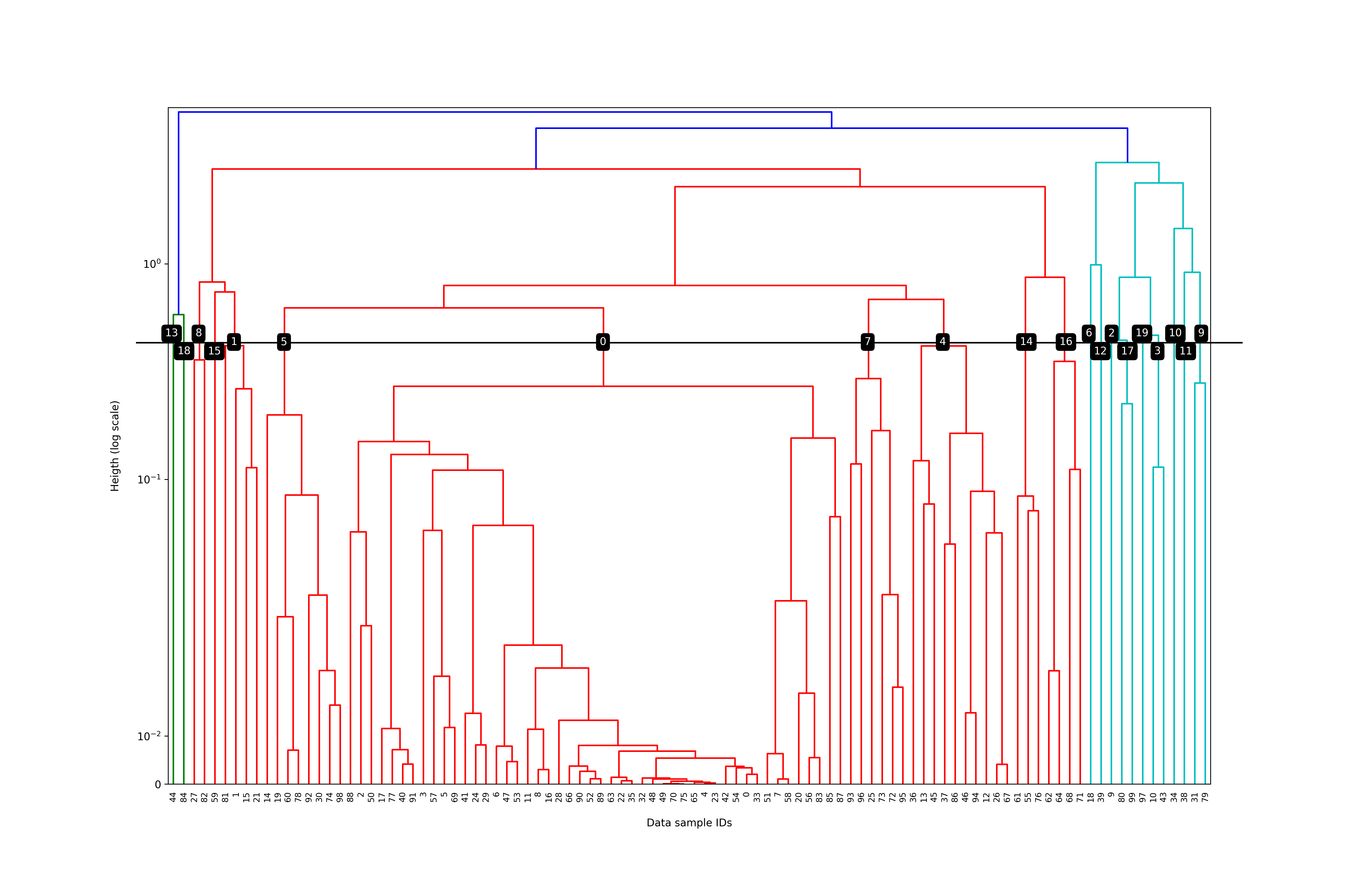
As shown below, the output is a numpy array of 100 elements, assigning one cluster ID to each input vector (of 4 dimensions, see above). Note that the ID of the resulting clusters go from 0 to 19 in this case. The resulting clustering is unbalanced, i.e. containing a big cluster (where the number of data samples is 48), and many small clusters (each containing very few data samples, 9 of them containing a single data sample). As result, the range of cluster sizes goes from 1 to 48, showing a standard deviation of 10.17 data samples.
Type of the standard clustering result: <class 'numpy.ndarray'>
Shape of the standard clustering result (one cluster id per data sample): (100, 1)
First 10 rows of the standard clustering result (one cluster id per sample):
[0 1 0 0 0 0 0 0 0 2] ...
Total number of resulting clusters = 20
For each resulting cluster: Cluster ID
[ 0  1  2  3  4  5  6  7  8  9 10 11 12 13 14 15 16 17 18 19]
For each resulting cluster: Count of data samples
[48  4  1  2 10  8  1  6  2  2  1  1  1  1  3  1  4  2  1  1]
Count of data samples per cluster: mean = 5, max = 48, min = 1, std = 10.17
The following figure illustrates visually the resulting clustering by using the standard tree cut. The black line shows the height at which the cut (i.e. pruning) is performed (which is identical for all clusters). The resulting cluster IDs are depicted within the black squares (i.e. numbers in white represent the obtained cluster IDs). As result, the cluster ID 0 contains 48 elements (almost half of the data samples), an issue which we try to address with our proposed method.
A more balanced clustering is then attempted by using the balanced ward tree method, in which the maximum number of data samples within each cluster is set to 10.
[balanced_cut_cluster_id, balanced_cut_cluster_level] = cut_tree_balanced(Z, 10, verbose=False)
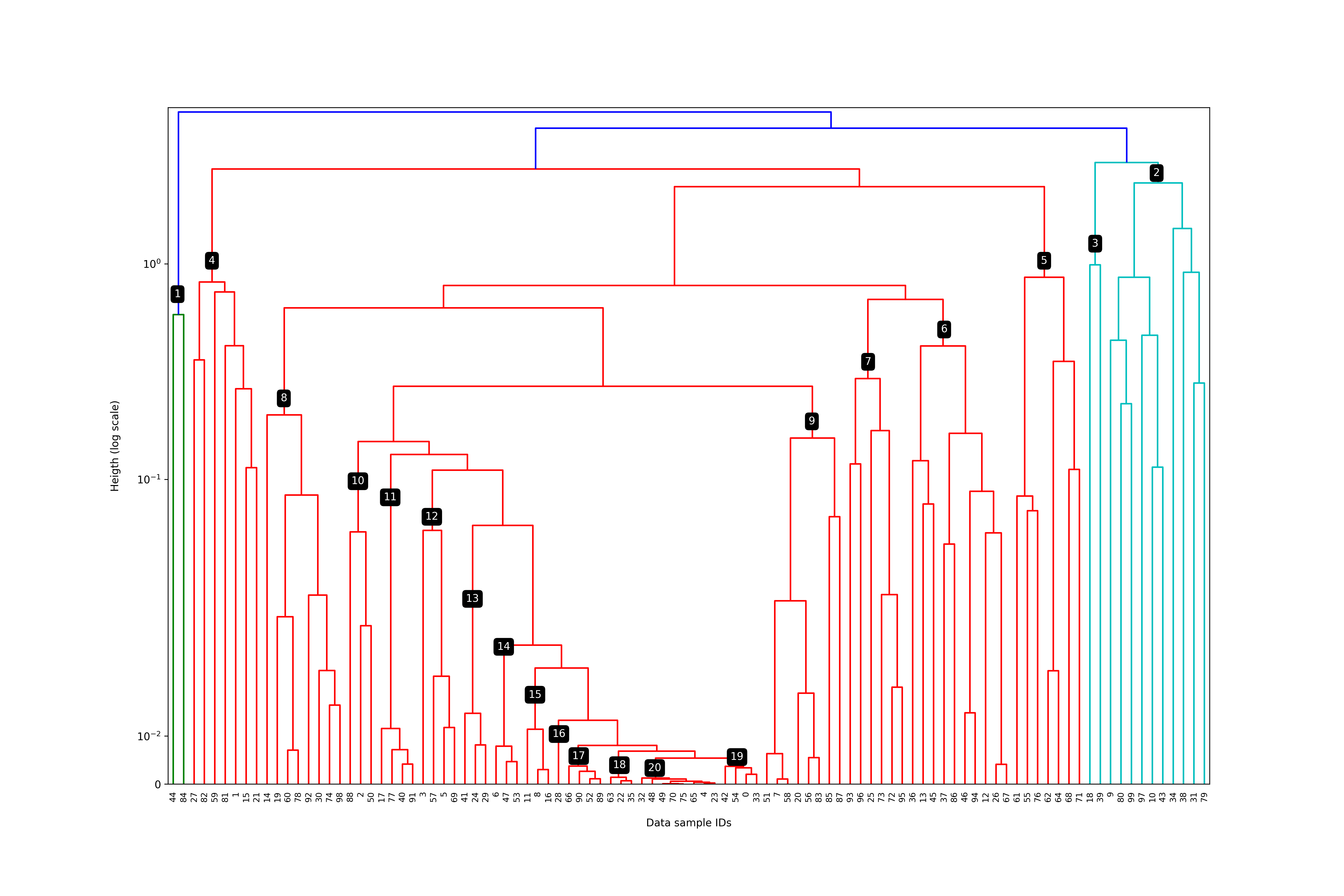
We get two results from the new function: (1) a list of integers containing for each input sample its corresponding cluster id, and (2) a list of strings containing for each input sample its corresponding cluster tree level (see above section for further information). Note that the ID of the resulting clusters go from 1 to 20 in this case, i.e. the number of resulting clusters (20) is identical to the previous one. Importantly, the resulting clustering is more balanced than the standard one (for an equal number of resulting clusters), since the range of cluster sizes goes from 1 to 10, showing a standard deviation of 2.68 data samples.
Type of the balanced clustering result (id): <class 'numpy.ndarray'>
Shape of the balanced clustering result (one cluster id per data sample): (100,)
First 10 rows of the balanced clustering result (one cluster id per sample):
[19  4 10 12 20 12 14  9 15  2] ...

Type of the balanced clustering result (level): <class 'numpy.ndarray'>
Shape of the balanced clustering result (level) (one array per data sample): (100,)
First 10 rows of the balanced clustering result (level) (one array per sample):
[array([0, 0, 0, 0, 0, 0, 0, 0, 0, 0, 0, 0, 0, 0, 0, 0, 0, 1])
 array([0, 0, 0, 1]) array([0, 0, 0, 0, 0, 0, 0, 0, 1])
 array([0, 0, 0, 0, 0, 0, 0, 0, 0, 0, 1])
 array([0, 0, 0, 0, 0, 0, 0, 0, 0, 0, 0, 0, 0, 0, 0, 0, 0, 0])
 array([0, 0, 0, 0, 0, 0, 0, 0, 0, 0, 1])
 array([0, 0, 0, 0, 0, 0, 0, 0, 0, 0, 0, 0, 1])
 array([0, 0, 0, 0, 0, 0, 0, 1])
 array([0, 0, 0, 0, 0, 0, 0, 0, 0, 0, 0, 0, 0, 1]) array([0, 0, 1, 0])] ...

Total number of resulting clusters = 20
For each resulting cluster: Cluster ID
[ 1  2  3  4  5  6  7  8  9 10 11 12 13 14 15 16 17 18 19 20]
For each resulting cluster: Count of data samples
[ 2 10  2  7  7 10  6  8  8  3  4  4  3  3  3  1  4  3  4  8]
Count of data samples per cluster: mean = 5, max = 10, min = 1, std = 2.68
The following figure illustrates visually the resulting balanced clustering. Again, the resulting cluster IDs are depicted within the black squares (i.e. numbers in white represent the obtained cluster IDs). Now the tree level at which the clusters are selected (i.e. pruned) is different for each cluster ID, since the cluster search method is not only driven by the heigth (i.e. distance between clusters), but also by the number of samples contained within the clusters. Note for instance that cluster ID 1 is smaller (2 data samples) than cluster ID 17 (4 data samples), although the heigth at which it was pruned is much higher. As result, all clusters contain less or equal than a number of specific data samples (in this case 10), and therefore their size is less variable.
In conclusion, here we describe and implement a method which generates (for a similar number of resulting clusters) a more balanced outcome, i.e. building clusters of less variable size.
Related Work
There are several implemented methods following the same or a similar idea, i.e. performing a tree cut in which the resulting clusters are at different tree levels.
- Implementation of the same method within the scikit-network package (see source code of the cut_balanced function).
- The CRAN R package dynamicTreeCut (see GitHub repo and the paper) implements novel dynamic branch cutting methods for detecting clusters in a dendrogram depending on their shape.
- Translation of the dynamicTreeCut method to Python.
- The web based MLCut tool (see GitHub repo and the paper) provides interactive methods to cut the branches of the tree at multiple levels.

