Models of Motor Inhibition during Motor Imagery

The momimi package implements different versions of the “threshold modulation model” (TMM3/TMM4) of motor imagery and provides fitting and plotting utilities.

Installation

You can install the latest stable version of the package from GitHub with:

# install.packages("devtools")
devtools::install_github(repo = "lnalborczyk/momimi", build_vignettes = TRUE)

Usage

Simulating and plotting data

We start by simulating some data (here, 100 observations or RTs and MTs).

library(tidyverse)
library(momimi)

simulated_data <- model(
    nsims = 100, nsamples = 2000,
    exec_threshold = 1.1, imag_threshold = 0.55,
    peak_time = log(0.5), curvature = 0.5,
    model_version = "TMM3",
    full_output = TRUE
    )

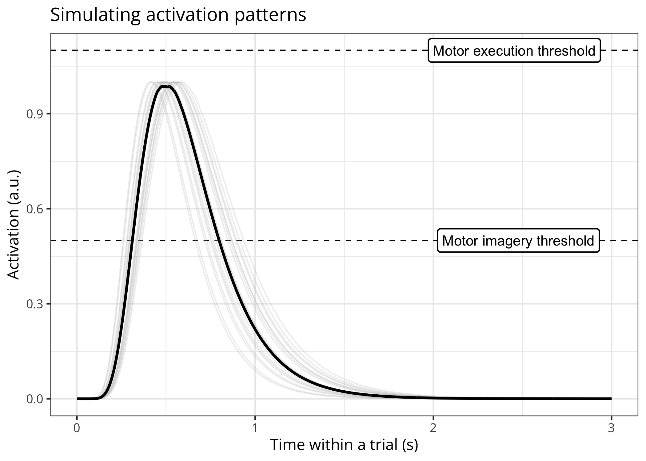
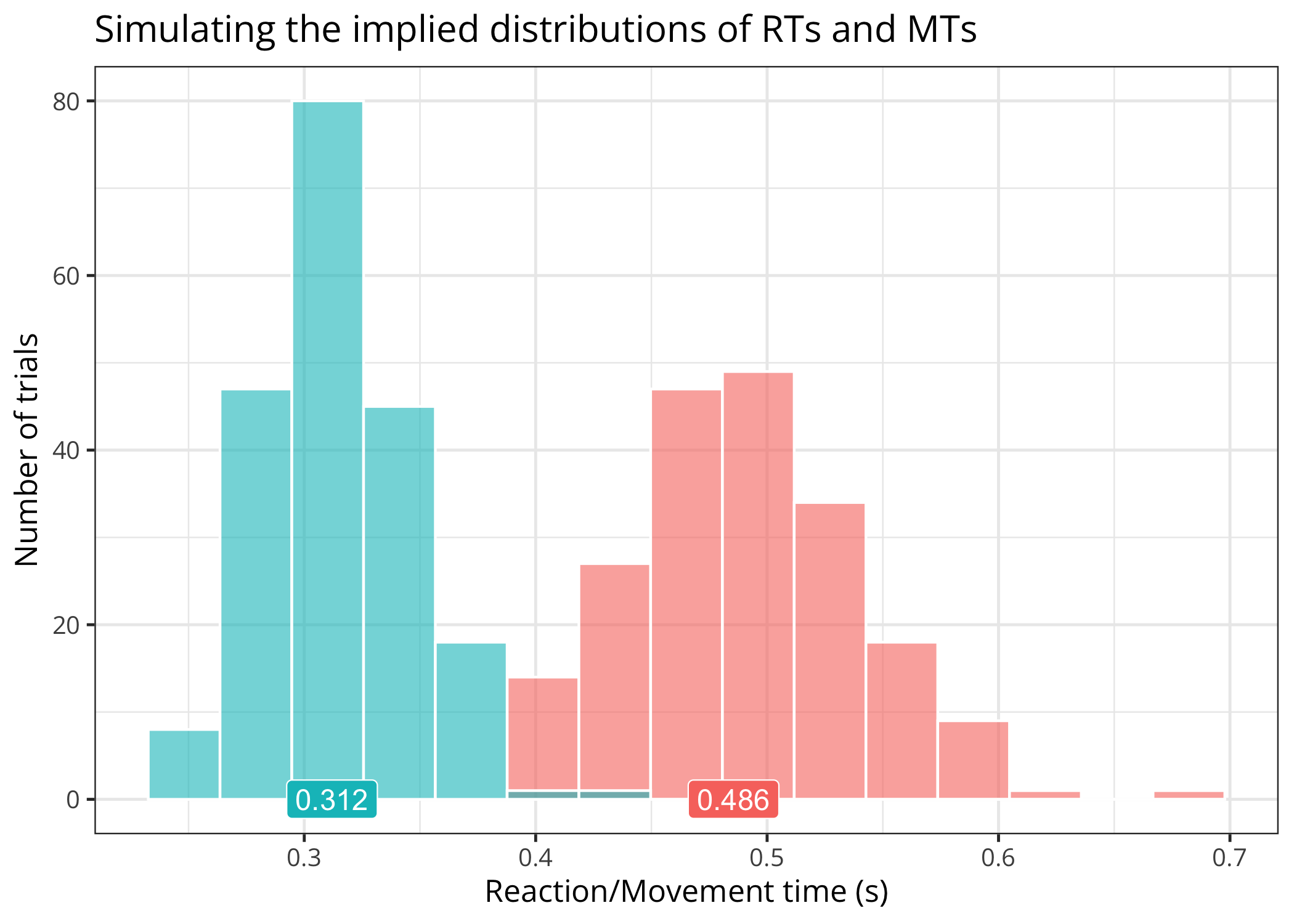
We can plot the underlying activation function and the implied distributions of RTs and MTs.

# plotting only the latent function(s)
plot(x = simulated_data, method = "functions")

# plotting only the distributions of RTs/MTs distributions
plot(x = simulated_data, method = "distributions")

Fitting the models

We can also use the model to generate realistic data from known parameter values and then fit the model (below, the 3-parameter version of the TMM) to these data to try recovering the original parameter values.

# plausible "true" parameter values in the TMM3
# parameters are the motor execution threshold, the peak time, and the curvature
true_pars <- c(1.1, 0.5, 0.4)

# simulating data using these parameter values
simulated_data <- simulating(
    nsims = 200,
    nsamples = 3000,
    true_pars = true_pars,
    action_mode = "imagined",
    model_version = "TMM3"
    )

# displaying the first ten rows of these data
head(x = simulated_data, n = 10)
#>    reaction_time movement_time action_mode
#> 1      0.3463210     0.5775052    imagined
#> 2      0.2916296     0.3477735    imagined
#> 3      0.3313592     0.4388002    imagined
#> 4      0.2302411     0.5789106    imagined
#> 5      0.2832451     0.5234344    imagined
#> 6      0.3649216     0.3350144    imagined
#> 7      0.3472452     0.6709369    imagined
#> 8      0.2788206     0.4660134    imagined
#> 9      0.3314475     0.6250139    imagined
#> 10     0.4021022     0.4734235    imagined

We fit the model and use realistic constraints (e.g., the RT/MT should be no less than 0.1s and no more than 2 seconds) on the initial parameter values (by setting initial_pop_constraints = TRUE) to facilitate convergence (fitting can take a while).

# fitting the model
results <- fitting(
    data = simulated_data,
    nsims = 200,
    error_function = "g2",
    method = "DEoptim",
    model_version = "TMM3",
    lower_bounds = c(1.0, 0.3, 0.2),
    upper_bounds = c(1.4, 0.7, 0.6),
    initial_pop_constraints = TRUE,
    nstudies = 200,
    rt_contraints = range(simulated_data$reaction_time),
    mt_contraints = range(simulated_data$movement_time),
    maxit = 100
    )

# fitting summary
summary(results)
#> 
#> ***** summary of DEoptim object ***** 
#> best member   :  1.13808 0.50313 0.41482 
#> best value    :  0.00876 
#> after         :  100 generations 
#> fn evaluated  :  26664 times 
#> *************************************

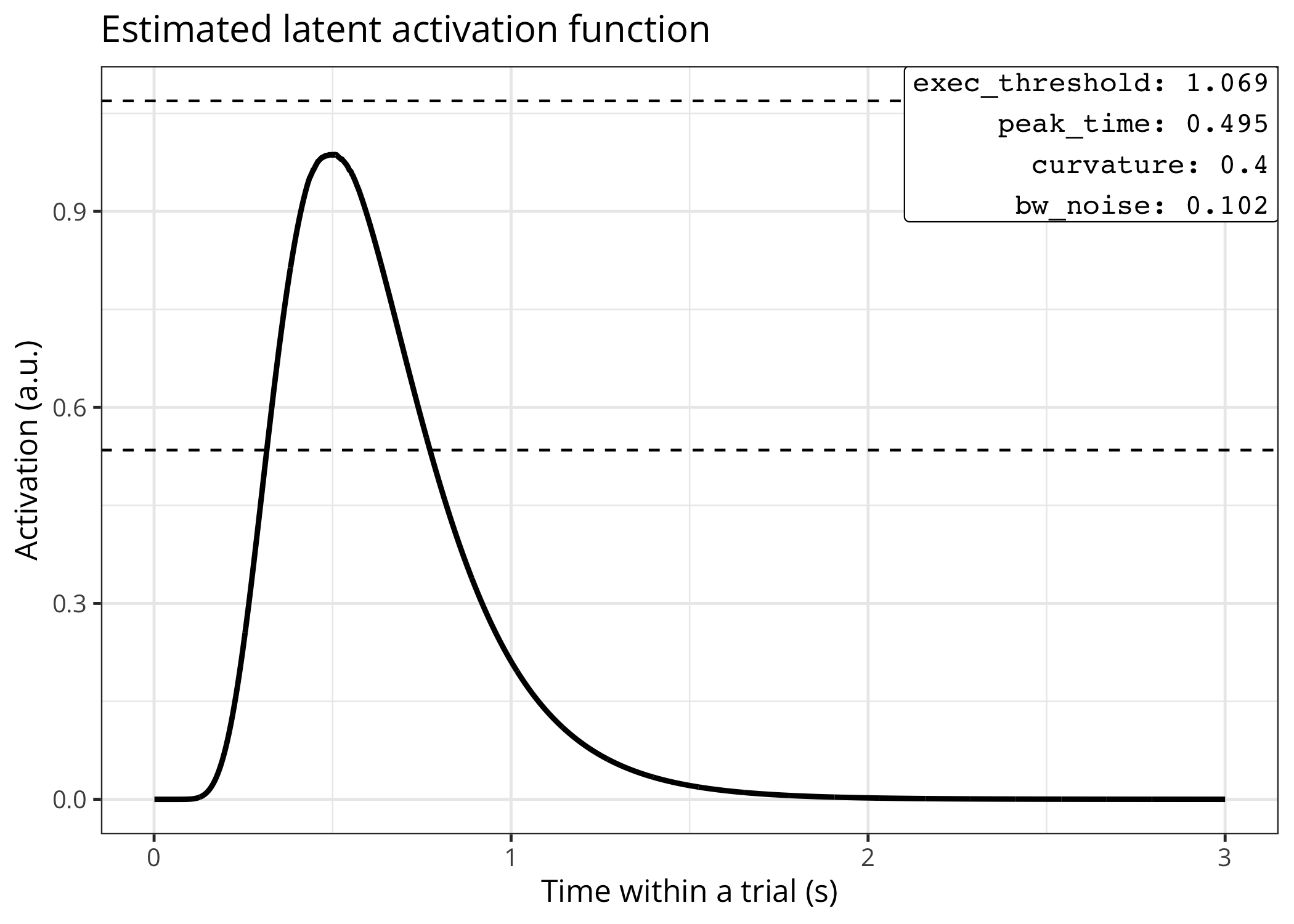
We can then plot the underlying (latent) function(s). Note that this returns a ggplot2 object that can be subsequently modified.

plot(x = results, method = "latent", model_version = "TMM3") +
    labs(title = "Example of latent activation function")

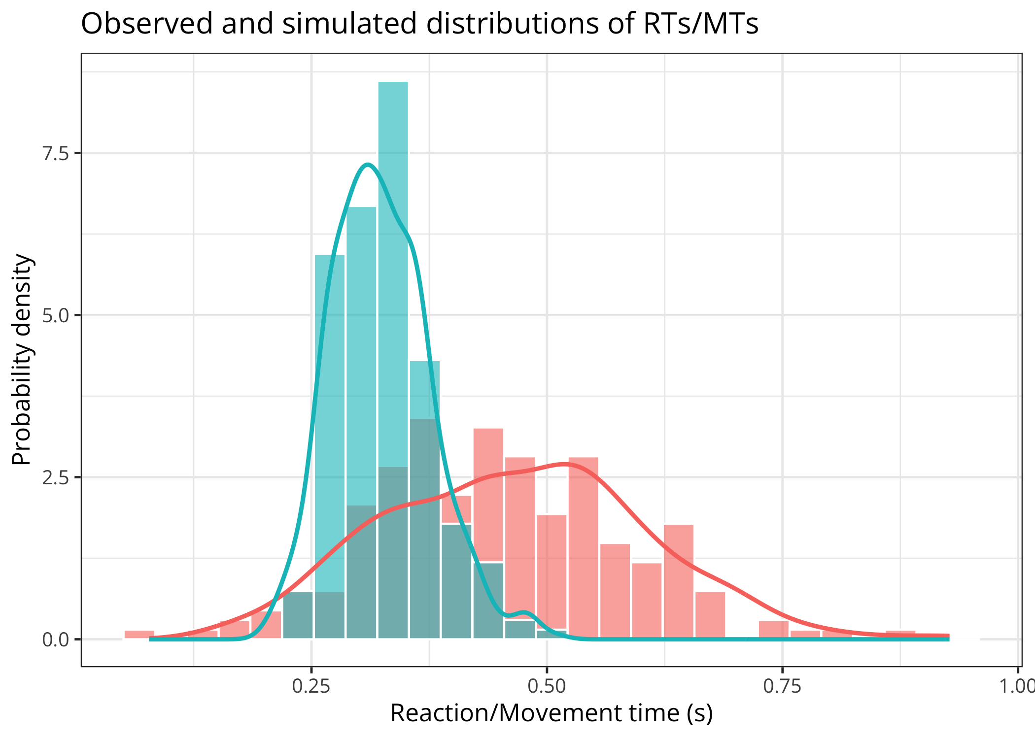
We can also do “predictive checks” by comparing the data used to fit the model to data simulated from the model using the estimated parameter values.

plot(
    x = results, original_data = simulated_data,
    method = "ppc", model_version = "TMM3", action_mode = "imagined"
    )

We can also do another form of “predictive check” by comparing the quantile values of the original and simulated data.

plot(
    x = results, original_data = simulated_data,
    method = "quantiles", model_version = "TMM3", action_mode = "imagined"
    )

We can also visualise the trajectory in parameter space during optimisation interactively using plotly (not shown below, but you should try this).

plot(x = results, method = "optimisation")

References

Nalborczyk, L., Longcamp, M., Gajdos, T., Servant, M. & Alario, F.‐X. (in preparation). Modelling the onset and duration of imagined actions: Assessing a novel algorithmic model of motor imagery.

Nalborczyk, L., Longcamp, M., Gajdos, T., Servant, M. & Alario, F.‐X. (2024). Towards formal models of inhibitory mechanisms involved in motor imagery: A commentary on Bach et al. (2022). Psychological Research, 1‐4. https://doi.org/10.1007/s00426-023-01915-8. Preprint available at https://psyarxiv.com/tz6x2/.

Getting help

If you encounter a bug or have a question please file an issue with a minimal reproducible example on GitHub.