README
Pierre Gaillard, Yannig Goude
- Setting: when is the package
operauseful? - Installation
- Example: predict the weekly electricity consumption.
- Meta
opera is a R package that provides several algorithms to perform robust online prediction of time series with the help of expert advice. In this vignette, we provide an example of how to use the package.
Setting: when is the package opera useful?
Consider a sequence of real bounded observations 


opera implements several algorithms of the online learning literature that form predictions 
What are the most important functions?
The package opera provides three important functions: mixture to build the algorithm object, predict to make a prediction by using the algorithm, and oracle to evaluate the performance of the experts and compare the performance of the combining algorithm.
Installation
opera is now available on CRAN, so you can install it with:
install.packages("opera")You can also install the development version of opera with the package devtools:
install.packages("devtools")
devtools::install_github("dralliag/opera")
You may be asked to install additional necessary packages. You can install the package vignette by setting the option: build_vignettes = TRUE.
Example: predict the weekly electricity consumption.
Here, we provide a concrete example on how to use the package. To do so, we consider an electricity forecasting data set that includes weekly observations of the French electric load together with several covariates: the temperature, calendar information, and industrial production indexes. The data set is provided by the French National Institute of Statistics and Economic Studies (Insee).
The data set
First, we load the data and we cut it into two subsets: a training set used to build the experts (base forecasting methods) and a testing set (here the last two years) used to evaluate the performance and to run the combining algorithms.
data(electric_load)
attach(electric_load)
idx_data_test <- 620:nrow(electric_load)
data_train <- electric_load[-idx_data_test, ]
data_test <- electric_load[idx_data_test, ]
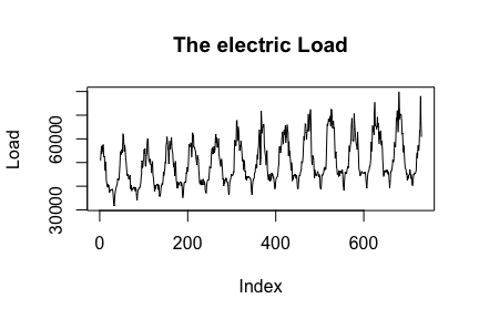
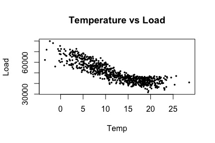
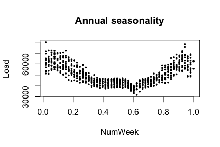
The data is displayed in the following figures.
plot(Load, type = "l", main = "The electric Load")Here, we build three base forecasting methods to be combined later.
- A generalized additive model using the
mgcvpackage:
library(mgcv)
gam.fit <- gam(Load ~ s(IPI) + s(Temp) + s(Time, k=3) +
                 s(Load1) + as.factor(NumWeek), data = data_train)
gam.forecast <- predict(gam.fit, newdata = data_test)- A medium term generalized additive model followed by an autoregressive short-term correction.
# medium term model
medium.fit <- gam(Load ~ s(Time,k=3) + s(NumWeek) + s(Temp) + s(IPI), data = data_train)
electric_load$Medium <- c(predict(medium.fit), predict(medium.fit, newdata = data_test))
electric_load$Residuals <- electric_load$Load - electric_load$Medium

# autoregressive correction
ar.forecast <- numeric(length(idx_data_test))
for (i in seq(idx_data_test)) {
  ar.fit <- ar(electric_load$Residuals[1:(idx_data_test[i] - 1)])
  ar.forecast[i] <- as.numeric(predict(ar.fit)$pred) + electric_load$Medium[idx_data_test[i]]
}- A gradient boosting model using
caretpackage
library(caret)
gbm.fit <- train(Load ~ IPI + IPI_CVS + Temp + Temp1 + Time + Load1 + NumWeek,
                 data = data_train, method = "gbm")
gbm.forecast <- predict(gbm.fit, newdata = data_test)
Once the expert forecasts have been created (note that they can also be formed online), we build the matrix of expert and the time series to be predicted online
Y <- data_test$Load
X <- cbind(gam.forecast, ar.forecast, gbm.forecast)
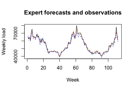
matplot(cbind(Y, X), type = "l", col = 1:6, ylab = "Weekly load",
xlab = "Week", main = "Expert forecasts and observations")To evaluate the performance of the experts and see if the aggregation rules may perform well, you can look at the oracles (rules that are used only for analysis and cannot be design online).
oracle.convex <- oracle(Y = Y, experts = X, loss.type = "square", model = "convex")
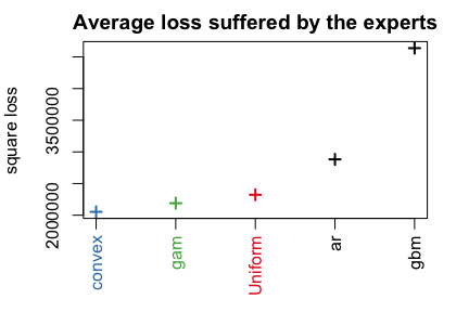
plot(oracle.convex)The parameter loss.type defines the evaluation criterion. It can be either the square loss, the percentage loss, the absolute loss, or the pinball loss to perform quantile regression.
The parameter model defines the oracle to be calculated. Here, we computed the best fixed convex combination of expert (i.e., with non-negative weights that sum to one).
Aggregate the experts online using one of the possible aggregation procedures
The first step consists in initializing the algorithm by defining the type of algorithm (Ridge regression, exponentially weighted average forecaster,...), the possible parameters, and the evaluation criterion. If no parameter is defined by the user, all parameters will be calibrated online by the algorithm. Bellow, we define the ML-Poly algorithm, evaluated by the square loss.
MLpol0 <- mixture(model = "MLpol", loss.type = "square")Then, you can perform online predictions by using the predict method. At each time, step the aggregation rule forms a new prediction and update the procedure.
MLpol <- MLpol0
for (i in 1:length(Y)) {
  MLpol <- predict(MLpol, newexperts = X[i, ], newY = Y[i])
}
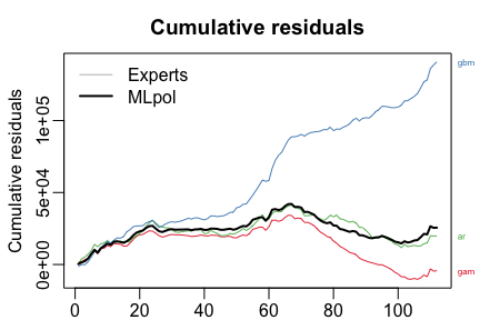
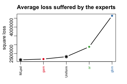
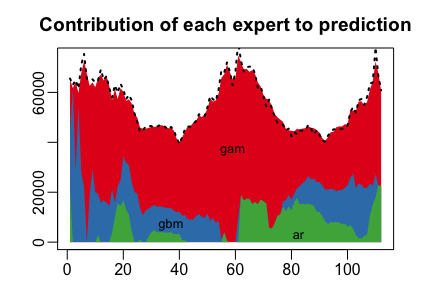
The results can be displayed with method summary and plot.
summary(MLpol)
#> Aggregation rule: MLpol
#> Loss function:  square loss
#> Gradient trick:  TRUE
#> Coefficients:
#>    gam    ar gbm
#>  0.631 0.369   0
#>
#> Number of experts:  3
#> Number of observations:  112
#> Dimension of the data:  1
#>
#>         rmse   mape
#> MLpol   1460 0.0189
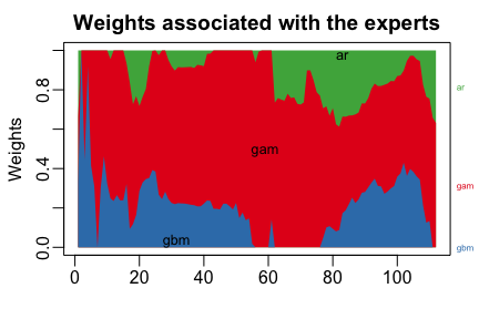
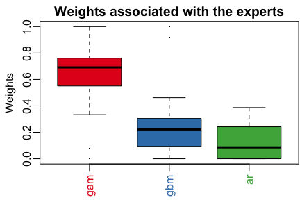
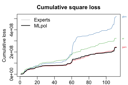
#> Uniform 1520 0.0197plot(MLpol, pause = TRUE, col = brewer.pal(3,name = "Set1"))- by giving the whole time series to
predictspecifyingonline = TRUEto perform online prediction.
MLpol <- predict(MLpol0, newexpert = X, newY = Y, online = TRUE)- or directly to the function mixture, when building the aggregation rule
MLpol <- mixture(Y = Y, experts = X, model = "MLpol", loss.type = "square")Meta
- Please report any issues or bugs.
- License: LGPL


