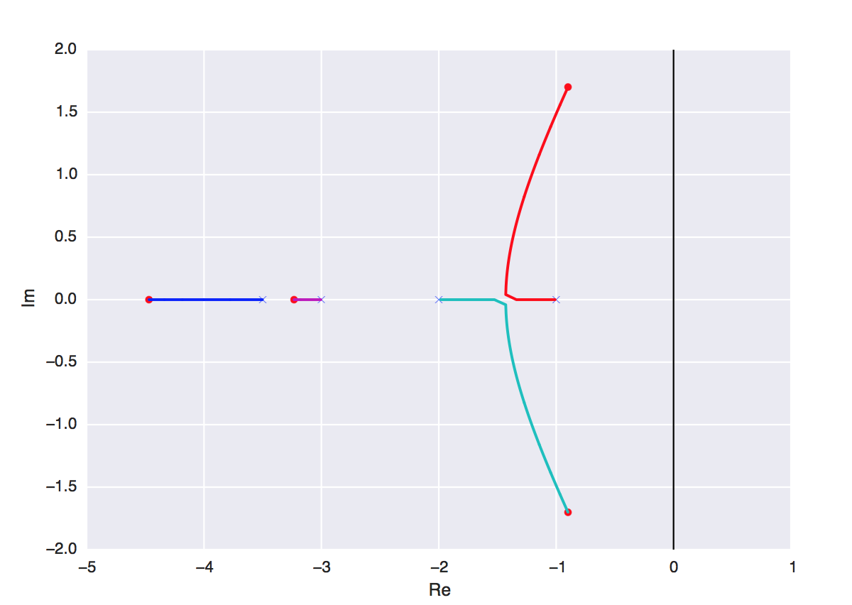
This is a fun little weekend project I worked on for my Modern Control Theory class.
It is a Python implementation of the Root Locus Design Method. It plots the location of the roots of the characteristic equation of the closed-loop transfer function as the gain K is varied from 0 to infinity.
Enter the coefficients of the numerator and denominator of the open loop transfer function as lists num = [] and denum = []. The denominator must have all coefficients entered (even the terms with 0 coefficients) but it doesn't have to be explicitly written out for the numerator.
Now invoke the transfer_function method, compute the roots of the TF using compute_roots, and finally plot with plot_root_locus.
Example
num = [1]
denum = [1, 3, 2, 0]

GH = transfer_function(num, denum)

# create a list of evenly spaced gains
gains = np.linspace(0.0, 10.0, num=500)

# compute and plot root-locus
roots = compute_roots(GH, gains)
fig, ax = plot_root_locus(gains, roots)
plt.show()- python-control - helped me get a sense of how to go about the problem.
- Bicycle Control Design - great blog post
