Complete Regression - Lab

Introduction

By now, you have created all the necessary functions to calculate the slope, intercept, best-fit line, prediction, and visualizations. In this lab you will put them all together to run a regression experiment and calculate the model loss.

Objectives

You will be able to:

Perform a linear regression using self-constructed functions
Calculate the coefficient of determination using self-constructed functions
Use the coefficient of determination to determine model performance

The formulas

Slope: $\hat m = \dfrac{\overline{x}*\overline{y}-\overline{xy}}{(\overline{x})^2-\overline{x^2}}$

Intercept: $ \hat c = \bar{y} - \hat m\bar{x}$

Prediction: $\hat{y} = \hat mx + \hat c$

R-Squared: $ R^2 = 1- \dfrac{SS_{RES}}{SS_{TOT}} = 1 - \dfrac{\sum_i(y_i - \hat y_i)^2}{\sum_i(y_i - \overline y_i)^2} $

Use the Python functions created earlier to implement these formulas to run a regression analysis using x and y as input variables.

# Combine all the functions created so far to run a complete regression experiment. 
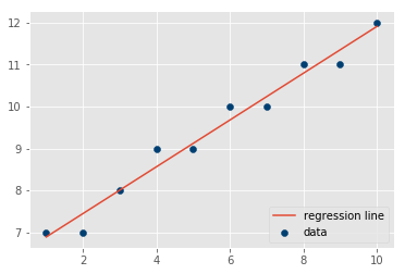
# Produce an output similar to the one shown below. 

X = np.array([1, 2, 3, 4, 5, 6, 7, 8, 9, 10], dtype=np.float64)
Y = np.array([7, 7, 8, 9, 9, 10, 10, 11, 11, 12], dtype=np.float64)

# Basic Regression Diagnostics
# ----------------------------
# Slope: 0.56
# Y-Intercept: 6.33
# R-Squared: 0.97
# ----------------------------
# Model: Y = 0.56 * X + 6.33

Basic Regression Diagnostics
----------------------------
Slope: 0.56
Y-Intercept: 6.33
R-Squared: 0.97
----------------------------
Model: Y = 0.56 * X + 6.33

Make Predictions

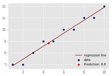
Predict and plot the value of y using regression line above for a new value of $x = 4.5$.

# Make prediction for x = 4.5 and visualize on the scatter plot

Level up - Optional

Load the "heightweight.csv" dataset. Use the height as an independent and weight as a dependent variable and draw a regression line to data using your code above. Calculate your R-Squared value for the model and try to predict new values of y.

Summary

In this lab, we ran a complete simple regression analysis experiment using functions created so far. Next up, you'll learn how you can use Python's built-in modules to perform similar analyses with a much higher level of sophistication.