In the previous lesson, we saw that the Kolmogorov–Smirnov statistic quantifies a distance between the empirical distribution function of the sample and the cumulative distribution function of the reference distribution, or between the empirical distribution functions of two samples. In this lab, we shall see how to perform this test in Python.
In this lab you will:
- Calculate a one- and two-sample Kolmogorov-Smirnov test
- Interpret the results of a one- and two-sample Kolmogorov-Smirnov test
- Compare K-S test to visual approaches for testing for normality assumption
Let's import the necessary libraries and generate some data. Run the following cell:
import scipy.stats as stats
import statsmodels.api as sm
import numpy as np

import matplotlib.pyplot as plt
plt.style.use('ggplot')

# Create the normal random variables with mean 0, and sd 3
x_10 = stats.norm.rvs(loc=0, scale=3, size=10)
x_50 = stats.norm.rvs(loc=0, scale=3, size=50)
x_100 = stats.norm.rvs(loc=0, scale=3, size=100)
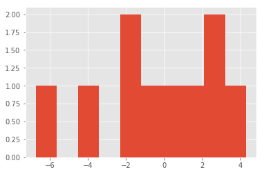
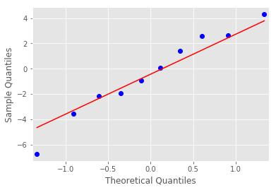
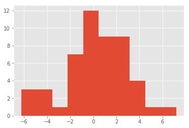
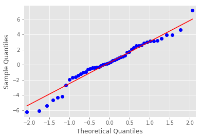
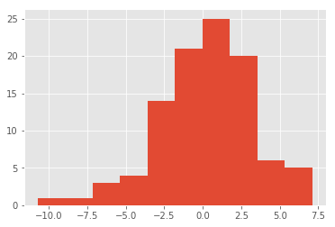
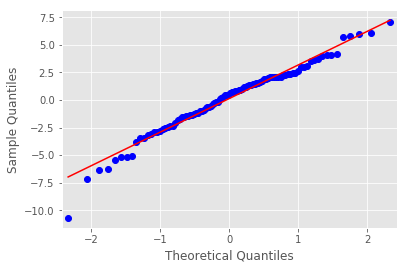
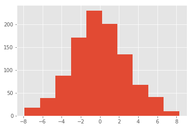
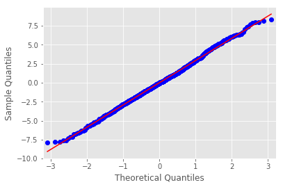
x_1000 = stats.norm.rvs(loc=0, scale=3, size=1000)Plot histograms and Q-Q plots of above datasets and comment on the output
- How good are these techniques for checking normality assumptions?
- Compare both these techniques and identify their limitations/benefits etc.
# Plot histograms and Q-Q plots for above datasets
x_10
x_50
x_100
x_1000
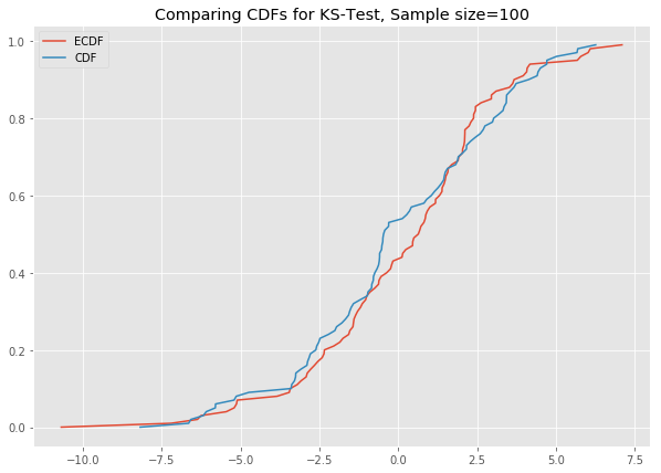
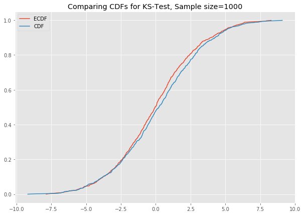
# Your comments here - Create a function to generate an empirical CDF from data
- Create a normal CDF using the same mean = 0 and sd = 3, having the same number of values as data
# You code here

def ks_plot(data):

    pass

# Uncomment below to run the test
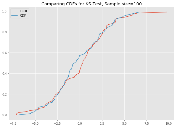
# ks_plot(stats.norm.rvs(loc=0, scale=3, size=100))
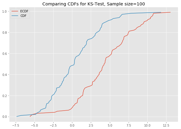
# ks_plot(stats.norm.rvs(loc=5, scale=4, size=100))
This is awesome. The difference between the two CDFs in the second plot shows that the sample did not come from the distribution which we tried to compare it against.
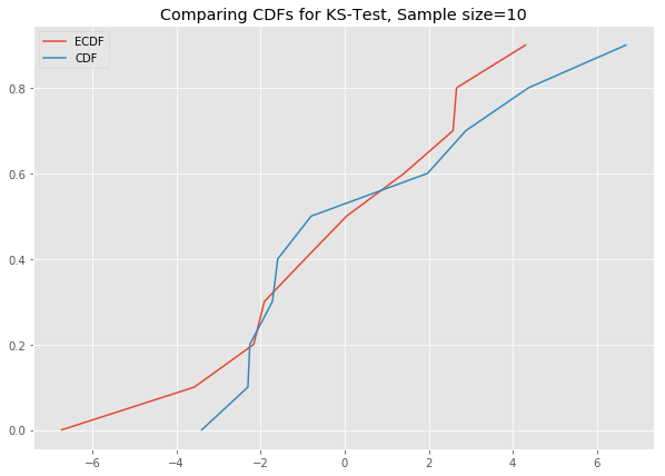
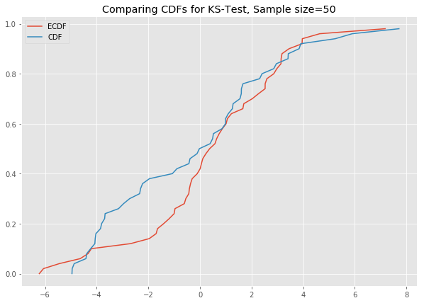
Now you can run all the generated datasets through the function ks_plot() and comment on the output.
# Your code here # Your comments here Let's run the Kolmogorov-Smirnov test, and use some statistics to get a final verdict on normality. We will test the hypothesis that the sample is a part of the standard t-distribution. In SciPy, we run this test using the function below:
scipy.stats.kstest(rvs, cdf, args=(), N=20, alternative='two-sided', mode='approx')Details on arguments being passed in can be viewed at this link to the official doc.
Run the K-S test for normality assumption using the datasets created earlier and comment on the output:
- Perform the K-S test against a normal distribution with mean = 0 and sd = 3
- If p < .05 we can reject the null hypothesis and conclude our sample distribution is not identical to a normal distribution
# Perform K-S test

# Your code here

# KstestResult(statistic=0.1377823669421559, pvalue=0.9913389045954595)
# KstestResult(statistic=0.13970573965633104, pvalue=0.2587483380087914)
# KstestResult(statistic=0.0901015276393986, pvalue=0.37158535281797134)
# KstestResult(statistic=0.030748345486274697, pvalue=0.29574612286614443)
KstestResult(statistic=0.1377823669421559, pvalue=0.9913389045954595)
KstestResult(statistic=0.13970573965633104, pvalue=0.2587483380087914)
KstestResult(statistic=0.0901015276393986, pvalue=0.37158535281797134)
KstestResult(statistic=0.030748345486274697, pvalue=0.29574612286614443)
# Your comments here Generate a uniform distribution and plot / calculate the K-S test against a uniform as well as a normal distribution:
x_uni = np.random.rand(1000)
# Try with a uniform distribution

# KstestResult(statistic=0.023778383763166322, pvalue=0.6239045200710681)
# KstestResult(statistic=0.5000553288071681, pvalue=0.0)
KstestResult(statistic=0.023778383763166322, pvalue=0.6239045200710681)
KstestResult(statistic=0.5000553288071681, pvalue=0.0)
# Your comments here A two-sample K-S test is available in SciPy using following function:
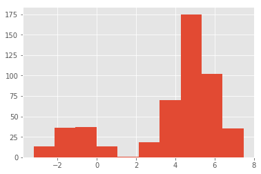
scipy.stats.ks_2samp(data1, data2)[source]Let's generate some bi-modal data first for this test:
# Generate binomial data
N = 1000
x_1000_bi = np.concatenate((np.random.normal(-1, 1, int(0.1 * N)), np.random.normal(5, 1, int(0.4 * N))))[:, np.newaxis]
plt.hist(x_1000_bi);
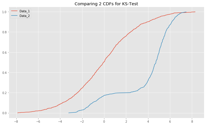
Plot the CDFs for x_1000_bimodal and x_1000 and comment on the output.
# Plot the CDFs
def ks_plot_2sample(data_1, data_2):
    '''
    Data entered must be the same size.
    '''
    pass

# Uncomment below to run
# ks_plot_2sample(x_1000, x_1000_bi[:,0])
# You comments here Run the two-sample K-S test on x_1000 and x_1000_bi and comment on the results.
# Your code here

# Ks_2sampResult(statistic=0.633, pvalue=4.814801487740621e-118)
# Your comments here In this lesson, we saw how to check for normality (and other distributions) using one- and two-sample K-S tests. You are encouraged to use this test for all the upcoming algorithms and techniques that require a normality assumption. We saw that we can actually make assumptions for different distributions by providing the correct CDF function into Scipy K-S test functions.
