Circuit Simulator

Requirements

Python 3.5+
Numpy
SciPy

Examples

See "examples.py" for the full example source code.

imports

    import cmath, math

    import circuit_sim
    from circuit_sim import bode_plot, interpolate, line_chart

DC Analysis

A resistor divider circuit:

    circuit = """    
        R R1    vcc     v_out   1k
        R       v_out   gnd     1kOhm
    
        vcc = 2.5v 
        """

Circuit Description Language Syntax:

Component names are optional - the first resistor is called R1, and the second one will get a name automatically assigned to
The "gnd" is automatically referenced to 0v
The units like "ohm" and "v" are optional

    circuit = circuit_sim.Circuit.build_from_string(circuit)
    circuit.dc_analysis()

    print("v_out =", circuit.get_variable("v_out")) # 1.25
    circuit.print_equations()                       # (0.002)(v_out) = 0.0025
    circuit.print_all_variables()                   # v_out = 1.25

Nonlinear DC Analysis

A diode in series with a resistor:

    circuit = """
        R           vcc     v1      0.1
        D my_diode  v1      gnd     i0=1e-5 m=3 v0=0.5

        vcc = 5v 
        """

The diode is modeled as I = (i0) * exp[m * (v - v0)]

    circuit = circuit_sim.Circuit.build_from_string(circuit)
    circuit.dc_analysis()
    circuit.print_all_variables()

    # v1 = 4.701818974760387
    # my_diode.internal_node = 0.33289232252030193
    # my_diode.current = 2.981810252396129

Using a calculator, you can verify that:

diode current: 2.982 = 0.00001 * exp ( 3 * (4.70812-0.5))
resistor current: 2.982 = (5 - 4.70182) / 0.1

Transient Simulation

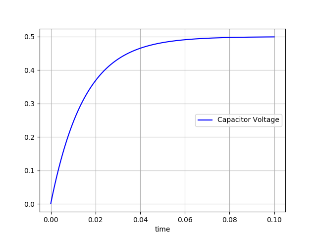
An RC circuit being charged:

    circuit = """
        R   vcc     v_out   1k
        R   v_out   gnd     1k
        C   v_out   gnd     30uF
        
        vcc = 1V
        """

To plot the "v_out":

    circuit = circuit_sim.Circuit.build_from_string(circuit)
    time_stamps, results = circuit.transient_simulation(0, 100e-3, ["v_out"])

    line_chart(x_label="time",
               #    [   x,            y,           graph_title   ]
               data=[time_stamps, results[0], "Capacitor Voltage"],
               legend_location="center right")

AC Sweep

A RC circuit:

    circuit = """
        R   vcc     v_out   1k
        R   v_out   gnd     1k
        C   v_out   gnd     1uF

        vcc = 1V
        """

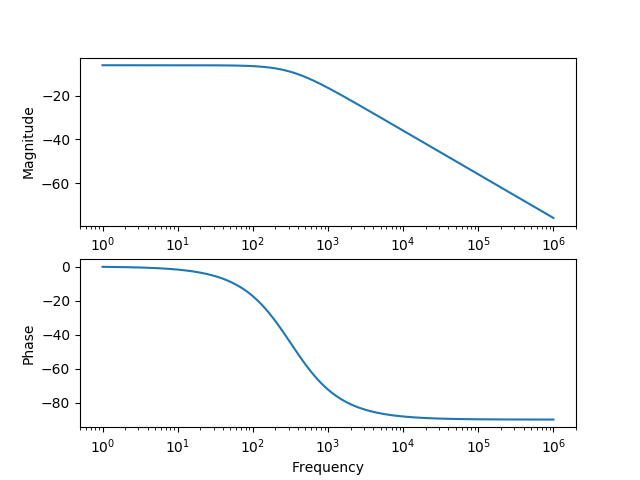
To make a Bode plot:

    circuit = circuit_sim.Circuit.build_from_string(circuit)
    freq, results = circuit.ac_sweep(["v_out"])
    bode_plot(freq, results[0])

Modifying Components during Transient Analysis

Example: buck converter output ripple modeling

A 12v to 5v buck converter model:

    circuit = """
            VG  vg      v_sw    gnd     12v
            L   L1      v_sw    v_out   50uH    v0=0    i0=5   
            C   C1      v_out   gnd     500uF   v0=5    i0=0
            R   R_load  v_out   gnd     1ohm
            """

Note the use of initial conditions for "L1" and "C1" to start the buck converter near it's steady state.

A buck converter applies a square wave into an LC circuit.

This is modeled by setting "vg" to 12v, then to 0v, then back to 12v, and so on.

    circuit = circuit_sim.Circuit.build_from_string(circuit)
    time_stamps, results = circuit.transient_simulation(0, 0, ["v_out"])

    on_time = 10e-6 * 5 / 12
    off_time = 10e-6 - on_time

    for i in range(0, 800):
        vg = circuit.get_component_for_modification("vg")
        vg.value = 12
        circuit.continue_transient_simulation(on_time, time_step=100e-9)

        vg = circuit.get_component_for_modification("vg")
        # The "get_component_for_modification" needs to be called again
        # and again because it registers the "vg" component as having
        # been modified.
        vg.value = 0
        circuit.continue_transient_simulation(off_time, time_step=100e-9)

This transient analysis will take some time to run.

The initial conditions put the circuit close to its stead state, but it's not exactly at the steady state. The long transient simulation is to put the model into its steady state.

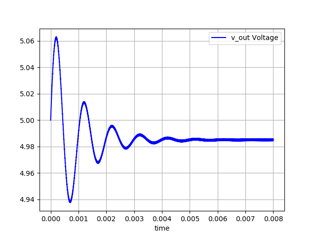
To see the output voltage during the long transient simulation:

    line_chart(x_label="time",
               data=[time_stamps, results[0], "v_out Voltage"],
               legend_location="upper right")

The steady state is not 5v due to approximations used during the transient simulation. The code is using a time step of 100ns, meaning 100 steps per 10us switching cycle. If a smaller time step is used, then the steady state output will be closer to 5v, at a cost of a longer simulation time.

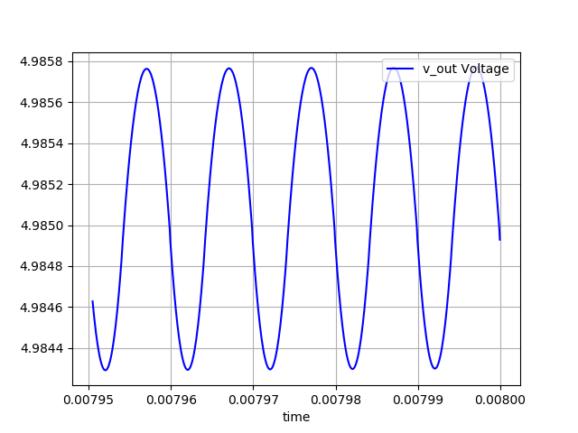
The switching ripple is visible if one zooms into the last few switching cycles:

    line_chart(x_label="time",
               data=[time_stamps[-500:], results[0][-500:], "v_out Voltage"],
               legend_location="upper right")

Digital Control

This example is rather long and not all of the code is provided below. The code involves three items:

the function "digital_buck()" is the example's entry point
the class "Controller" models the buck converter's digital controller
the function "run_buck_converter(...)" runs the buck circuit for a single switching cycle

This "README.md" file will only go over "digital_buck()", so import the other two items:

from examples import Controller, run_buck_converter

A 12v to 5v buck converter model:

    circuit = """
            VG  vg      v_sw    gnd     12v
            L   L1      v_sw    v_out   50uH   
            C   C1      v_out   gnd     500uF
            R   R_load  v_out   gnd     1ohm
            """

Unlike in the previous example, the "L1" and "C1" are initialized to close the operating point. In this example, these components start off at 0v.

To prepare for the simulation:

    circuit = circuit_sim.Circuit.build_from_string(circuit)
    time_stamps, results = circuit.transient_simulation(0, 0, ["v_out"])
    duty_cycle_data = []
    duty_cycle_data_t = []

    controller = Controller(circuit)

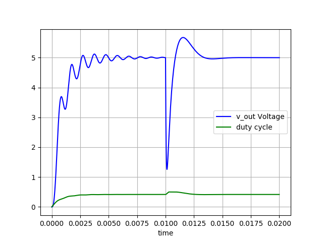
The duty cycle is not part of the circuit, so a separate list is allocated. The duty cycle is also not sampled at the same rate as the circuit, so a separate "_t" list is used to hold the time stamps. The code inside ""run_buck_converter(...)" simulates the circuit elements using 10 time steps per 10us switching cycle. During this same time period, there is only one duty cycle value, and only one duty timestamp, which is why the "duty_cycle_data[]" list is ten times shorter than the circuit simulation data.

To run the buck converter for 1000 cycles:

    # starting condition: 1 ohm load
    run_buck_converter(circuit, controller, duty_cycle_data,
                       duty_cycle_data_t, num_cycles=1000)

Next, change the load resistor and then run the buck converter for another 1000 cycles.

    # change load to 0.1 ohm
    r_load = circuit.get_component_for_modification("R_load")
    r_load.value = 0.1

    run_buck_converter(circuit, controller, duty_cycle_data,
                       duty_cycle_data_t, num_cycles=1000)

Plot the output voltage:

    line_chart(x_label="time",
               #    [   x,            y,        graph_title  ]
               data=[time_stamps, results[0], "v_out Voltage",
                     duty_cycle_data_t, duty_cycle_data, "duty cycle"],
                     legend_location="center right")

This is bad! Good thing this is a circuit simulator project and not a power supply project...

Improving the control

To keep the example simple, the code inside the "Controller" class is just using proportional control, and it's using voltage mode only.

In addition to more complex compensation schemes, current mode control can be implemented by reading the inductor current, using:

    i_L = self.__circuit.get_variable("L1.current")