louisyuzhe/Deep-Neural-Network-Image-Classification

Build a supervised learning deep neural network for Image Classification

Deep Neural Network for Image Classification: Application

Build a supervised learning deep neural network, and apply it to cat vs non-cat classification.

1 - Packages

Import packages

• numpy is the fundamental package for scientific computing with Python.
• matplotlib is a library to plot graphs in Python.
• h5py is a common package to interact with a dataset that is stored on an H5 file.
• PIL and scipy are used here to test the model with custom picture at the end.
• dnn_app_utils provides the functions implemented in the "Building_Deep_Neural_Network_from_scratch.ipynb"

import time
import numpy as np
import h5py
import matplotlib.pyplot as plt
import scipy
from PIL import Image
from scipy import ndimage
from dnn_app_utils_v3 import *

%matplotlib inline
plt.rcParams['figure.figsize'] = (5.0, 4.0) # set default size of plots
plt.rcParams['image.interpolation'] = 'nearest'
plt.rcParams['image.cmap'] = 'gray'

%load_ext autoreload
%autoreload 2

np.random.seed(1)

2 - Dataset

("data.h5") contains: - a training set of m_train images labelled as cat (1) or non-cat (0) - a test set of m_test images labelled as cat and non-cat - each image is of shape (num_px, num_px, 3) where 3 is for the 3 channels (RGB).

train_x_orig, train_y, test_x_orig, test_y, classes = load_data()

# Example of a picture
index = 7
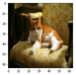
plt.imshow(train_x_orig[index])
print ("y = " + str(train_y[0,index]) + ". It's a " + classes[train_y[0,index]].decode("utf-8") +  " picture.")

y = 1. It's a cat picture.

# Explore dataset
m_train = train_x_orig.shape[0]
num_px = train_x_orig.shape[1]
m_test = test_x_orig.shape[0]

print ("Number of training examples: " + str(m_train))
print ("Number of testing examples: " + str(m_test))
print ("Each image is of size: (" + str(num_px) + ", " + str(num_px) + ", 3)")
print ("train_x_orig shape: " + str(train_x_orig.shape))
print ("train_y shape: " + str(train_y.shape))
print ("test_x_orig shape: " + str(test_x_orig.shape))
print ("test_y shape: " + str(test_y.shape))

Number of training examples: 209
Number of testing examples: 50
Each image is of size: (64, 64, 3)
train_x_orig shape: (209, 64, 64, 3)
train_y shape: (1, 209)
test_x_orig shape: (50, 64, 64, 3)
test_y shape: (1, 50)

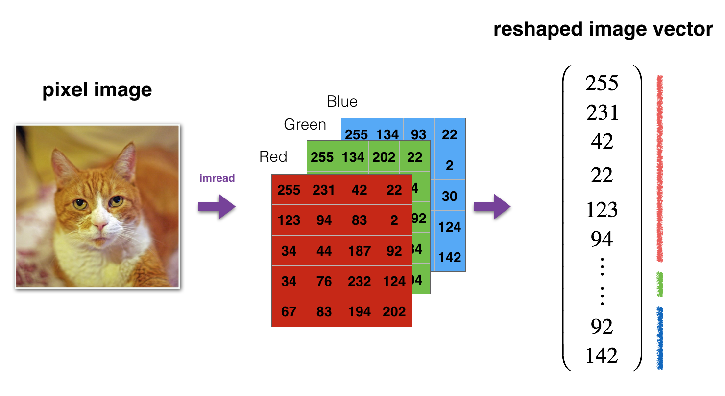
Reshape and standardize the images before feeding them to the network.

Figure 1: Image to vector conversion.

# Reshape the training and test examples
train_x_flatten = train_x_orig.reshape(train_x_orig.shape[0], -1).T   # The "-1" makes reshape flatten the remaining dimensions
test_x_flatten = test_x_orig.reshape(test_x_orig.shape[0], -1).T

# Standardize data to have feature values between 0 and 1.
train_x = train_x_flatten/255.
test_x = test_x_flatten/255.

print ("train_x's shape: " + str(train_x.shape))
print ("test_x's shape: " + str(test_x.shape))

train_x's shape: (12288, 209)
test_x's shape: (12288, 50)

$12,288$ equals $64 \times 64 \times 3$ which is the size of one reshaped image vector.

3 - Architecture of model

Build two different models:

• A 2-layer neural network
• An L-layer deep neural network

Then, compare the performance of these models, and also try out different values for $L$.

3.1 - 2-layer neural network

Figure 2: 2-layer neural network.
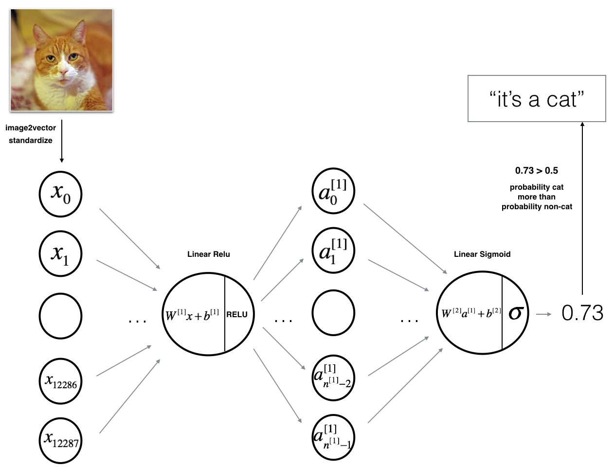
The model can be summarized as: ***INPUT -> LINEAR -> RELU -> LINEAR -> SIGMOID -> OUTPUT***.

Detailed Architecture of figure 2:

• The input is a (64,64,3) image which is flattened to a vector of size $(12288,1)$.
• The corresponding vector: $[x_0,x_1,...,x_{12287}]^T$ is then multiplied by the weight matrix $W^{[1]}$ of size $(n^{[1]}, 12288)$.
• Then add a bias term and take its relu to get the following vector: $[a_0^{[1]}, a_1^{[1]},..., a_{n^{[1]}-1}^{[1]}]^T$.
• Then repeat the same process.
• Multiply the resulting vector by $W^{[2]}$ and add intercept (bias).
• Finally, take the sigmoid of the result. If it is greater than 0.5, classify it to be a cat.

3.2 - L-layer deep neural network

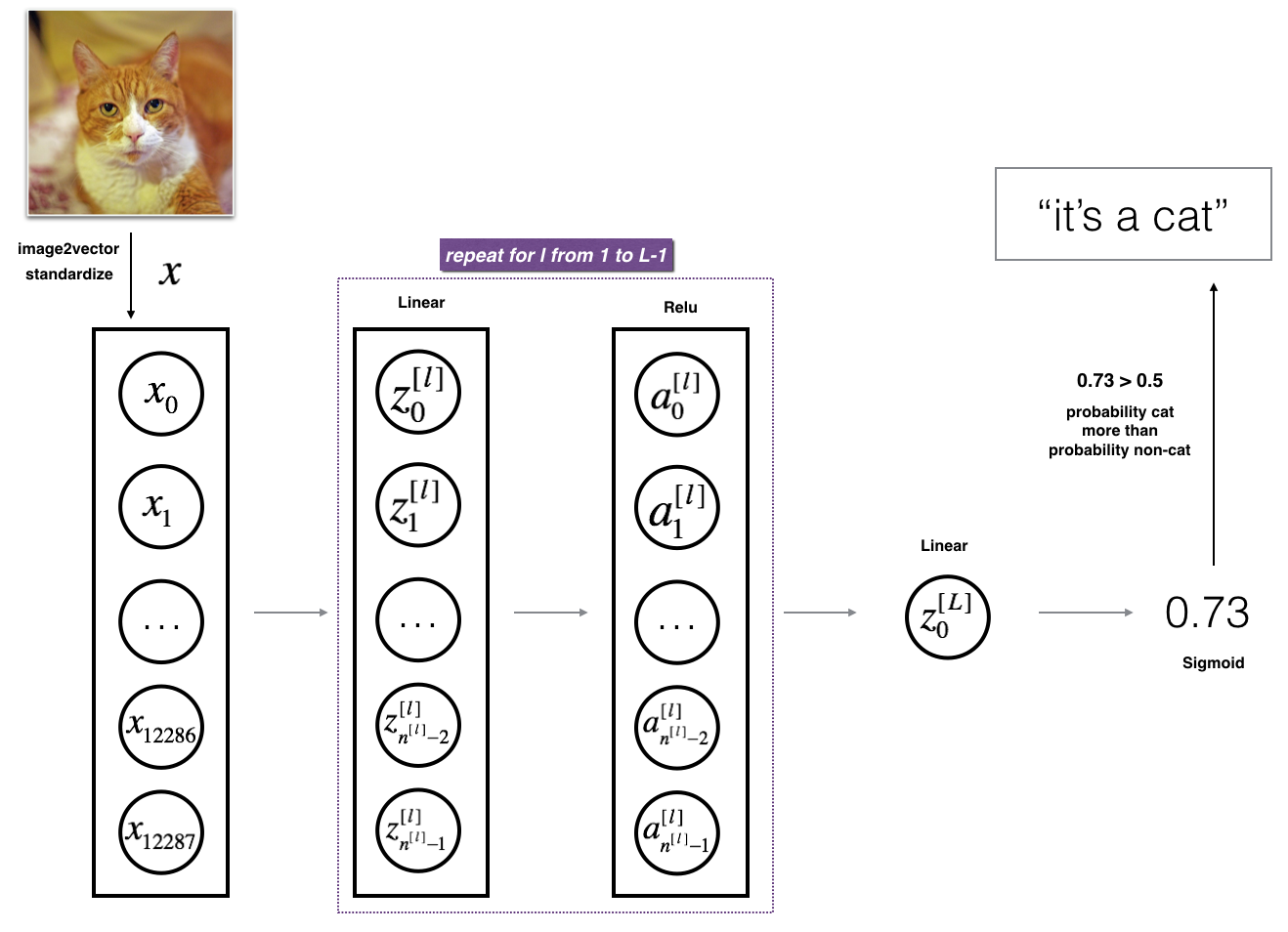
It is hard to represent an L-layer deep neural network with the above representation. However, here is a simplified network representation:

Figure 3: L-layer neural network.
The model can be summarized as: ***[LINEAR -> RELU] $\times$ (L-1) -> LINEAR -> SIGMOID***

Detailed Architecture of figure 3:

• The input is a (64,64,3) image which is flattened to a vector of size (12288,1).
• The corresponding vector: $[x_0,x_1,...,x_{12287}]^T$ is then multiplied by the weight matrix $W^{[1]}$ and then add the intercept $b^{[1]}$. The result is called the linear unit.
• Next, take the relu of the linear unit. This process could be repeated several times for each $(W^{[l]}, b^{[l]})$ depending on the model architecture.
• Finally, take the sigmoid of the final linear unit. If it is greater than 0.5, classify it to be a cat.

3.3 - General methodology

Deep Learning methodology to build the model: 1. Initialize parameters / Define hyperparameters 2. Loop for num_iterations: a. Forward propagation b. Compute cost function c. Backward propagation d. Update parameters (using parameters, and grads from backprop) 4. Use trained parameters to predict labels

4 - Two-layer neural network

Functions to build a 2-layer neural network with the following structure: LINEAR -> RELU -> LINEAR -> SIGMOID.

def initialize_parameters(n_x, n_h, n_y):
    ...
    return parameters
def linear_activation_forward(A_prev, W, b, activation):
    ...
    return A, cache
def compute_cost(AL, Y):
    ...
    return cost
def linear_activation_backward(dA, cache, activation):
    ...
    return dA_prev, dW, db
def update_parameters(parameters, grads, learning_rate):
    ...
    return parameters

### CONSTANTS DEFINING THE MODEL ####
n_x = 12288     # num_px * num_px * 3
n_h = 7
n_y = 1
layers_dims = (n_x, n_h, n_y)

# Implement two_layer_model

def two_layer_model(X, Y, layers_dims, learning_rate = 0.0075, num_iterations = 3000, print_cost=False):
    """
    Implements a two-layer neural network: LINEAR->RELU->LINEAR->SIGMOID.

    Arguments:
    X -- input data, of shape (n_x, number of examples)
    Y -- true "label" vector (containing 1 if cat, 0 if non-cat), of shape (1, number of examples)
    layers_dims -- dimensions of the layers (n_x, n_h, n_y)
    num_iterations -- number of iterations of the optimization loop
    learning_rate -- learning rate of the gradient descent update rule
    print_cost -- If set to True, this will print the cost every 100 iterations

    Returns:
    parameters -- a dictionary containing W1, W2, b1, and b2
    """

    np.random.seed(1)
    grads = {}
    costs = []                              # to keep track of the cost
    m = X.shape[1]                           # number of examples
    (n_x, n_h, n_y) = layers_dims

    # Initialize parameters dictionary
    parameters = initialize_parameters(n_x, n_h, n_y)

    # Get W1, b1, W2 and b2 from the dictionary parameters.
    W1 = parameters["W1"]
    b1 = parameters["b1"]
    W2 = parameters["W2"]
    b2 = parameters["b2"]

    # Loop (gradient descent)

    for i in range(0, num_iterations):

        # Forward propagation: LINEAR -> RELU -> LINEAR -> SIGMOID. Inputs: "X, W1, b1, W2, b2". Output: "A1, cache1, A2, cache2".
        A1, cache1 = linear_activation_forward(X, W1, b1, 'relu')
        A2, cache2 = linear_activation_forward(A1, W2, b2, 'sigmoid')

        # Compute cost
        cost = compute_cost(A2, Y)

        # Initializing backward propagation
        dA2 = - (np.divide(Y, A2) - np.divide(1 - Y, 1 - A2))

        # Backward propagation. Inputs: "dA2, cache2, cache1". Outputs: "dA1, dW2, db2; also dA0 (not used), dW1, db1".
        dA1, dW2, db2 = linear_activation_backward(dA2, cache2, 'sigmoid')
        dA0, dW1, db1 = linear_activation_backward(dA1, cache1, 'relu')

        # Set grads['dWl'] to dW1, grads['db1'] to db1, grads['dW2'] to dW2, grads['db2'] to db2
        grads['dW1'] = dW1
        grads['db1'] = db1
        grads['dW2'] = dW2
        grads['db2'] = db2

        # Update parameters.
        parameters = update_parameters(parameters, grads, learning_rate)

        # Retrieve W1, b1, W2, b2 from parameters
        W1 = parameters["W1"]
        b1 = parameters["b1"]
        W2 = parameters["W2"]
        b2 = parameters["b2"]

        # Print the cost every 100 training example
        if print_cost and i % 100 == 0:
            print("Cost after iteration {}: {}".format(i, np.squeeze(cost)))
        if print_cost and i % 100 == 0:
            costs.append(cost)

    # plot the cost

    plt.plot(np.squeeze(costs))
    plt.ylabel('cost')
    plt.xlabel('iterations (per hundreds)')
    plt.title("Learning rate =" + str(learning_rate))
    plt.show()

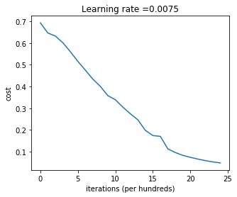
    return parameters

Train the parameters, the cost should be decreasing. It may take up to 5 minutes to run 2500 iterations.

parameters = two_layer_model(train_x, train_y, layers_dims = (n_x, n_h, n_y), num_iterations = 2500, print_cost=True)

Cost after iteration 0: 0.6930497356599888
Cost after iteration 100: 0.6464320953428849
Cost after iteration 200: 0.6325140647912677
Cost after iteration 300: 0.6015024920354665
Cost after iteration 400: 0.5601966311605747
Cost after iteration 500: 0.5158304772764729
Cost after iteration 600: 0.47549013139433255
Cost after iteration 700: 0.43391631512257495
Cost after iteration 800: 0.400797753620389
Cost after iteration 900: 0.3580705011323798
Cost after iteration 1000: 0.3394281538366411
Cost after iteration 1100: 0.3052753636196264
Cost after iteration 1200: 0.2749137728213018
Cost after iteration 1300: 0.24681768210614854
Cost after iteration 1400: 0.19850735037466094
Cost after iteration 1500: 0.17448318112556666
Cost after iteration 1600: 0.17080762978096128
Cost after iteration 1700: 0.11306524562164724
Cost after iteration 1800: 0.09629426845937152
Cost after iteration 1900: 0.08342617959726856
Cost after iteration 2000: 0.07439078704319078
Cost after iteration 2100: 0.06630748132267927
Cost after iteration 2200: 0.05919329501038164
Cost after iteration 2300: 0.05336140348560553
Cost after iteration 2400: 0.048554785628770115

predictions_train = predict(train_x, train_y, parameters)

Accuracy: 1.0

predictions_test = predict(test_x, test_y, parameters)

Accuracy: 0.72

Note: You may notice that running the model on fewer iterations (say 1500) gives better accuracy on the test set. This is called "early stopping". Early stopping is a way to prevent overfitting.

2-layer neural network has a performance of 72%. Let's see if we can do even better with an $L$-layer model.

5 - L-layer Neural Network

Build an $L$-layer neural network with the following structure: [LINEAR -> RELU]$\times$(L-1) -> LINEAR -> SIGMOID.

def initialize_parameters_deep(layers_dims):
    ...
    return parameters
def L_model_forward(X, parameters):
    ...
    return AL, caches
def compute_cost(AL, Y):
    ...
    return cost
def L_model_backward(AL, Y, caches):
    ...
    return grads
def update_parameters(parameters, grads, learning_rate):
    ...
    return parameters

### CONSTANTS ###
layers_dims = [12288, 20, 7, 5, 1] #  4-layer model

# L_layer_model

def L_layer_model(X, Y, layers_dims, learning_rate = 0.0075, num_iterations = 3000, print_cost=False):#lr was 0.009
    """
    Implements a L-layer neural network: [LINEAR->RELU]*(L-1)->LINEAR->SIGMOID.

    Arguments:
    X -- data, numpy array of shape (num_px * num_px * 3, number of examples)
    Y -- true "label" vector (containing 0 if cat, 1 if non-cat), of shape (1, number of examples)
    layers_dims -- list containing the input size and each layer size, of length (number of layers + 1).
    learning_rate -- learning rate of the gradient descent update rule
    num_iterations -- number of iterations of the optimization loop
    print_cost -- if True, it prints the cost every 100 steps

    Returns:
    parameters -- parameters learnt by the model. They can then be used to predict.
    """

    np.random.seed(1)
    costs = []                         # keep track of cost

    # Parameters initialization.
    parameters = initialize_parameters_deep(layers_dims)

    # Loop (gradient descent)
    for i in range(0, num_iterations):

        # Forward propagation: [LINEAR -> RELU]*(L-1) -> LINEAR -> SIGMOID.
        AL, caches = L_model_forward(X, parameters)

        # Compute cost.
        cost = compute_cost(AL, Y)

        # Backward propagation.
        grads = L_model_backward(AL, Y, caches)

        # Update parameters.
        parameters = update_parameters(parameters, grads, learning_rate)

        # Print the cost every 100 training example
        if print_cost and i % 100 == 0:
            print ("Cost after iteration %i: %f" %(i, cost))
        if print_cost and i % 100 == 0:
            costs.append(cost)

    # plot the cost
    plt.plot(np.squeeze(costs))
    plt.ylabel('cost')
    plt.xlabel('iterations (per hundreds)')
    plt.title("Learning rate =" + str(learning_rate))
    plt.show()

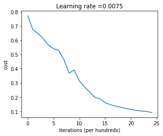
    return parameters

Now train the model as a 4-layer neural network. The cost should decrease on every iteration. It may take up to 5 minutes to run 2500 iterations.

parameters = L_layer_model(train_x, train_y, layers_dims, num_iterations = 2500, print_cost = True)

Cost after iteration 0: 0.771749
Cost after iteration 100: 0.672053
Cost after iteration 200: 0.648263
Cost after iteration 300: 0.611507
Cost after iteration 400: 0.567047
Cost after iteration 500: 0.540138
Cost after iteration 600: 0.527930
Cost after iteration 700: 0.465477
Cost after iteration 800: 0.369126
Cost after iteration 900: 0.391747
Cost after iteration 1000: 0.315187
Cost after iteration 1100: 0.272700
Cost after iteration 1200: 0.237419
Cost after iteration 1300: 0.199601
Cost after iteration 1400: 0.189263
Cost after iteration 1500: 0.161189
Cost after iteration 1600: 0.148214
Cost after iteration 1700: 0.137775
Cost after iteration 1800: 0.129740
Cost after iteration 1900: 0.121225
Cost after iteration 2000: 0.113821
Cost after iteration 2100: 0.107839
Cost after iteration 2200: 0.102855
Cost after iteration 2300: 0.100897
Cost after iteration 2400: 0.092878

pred_train = predict(train_x, train_y, parameters)

Accuracy: 0.985645933014

pred_test = predict(test_x, test_y, parameters)

Accuracy: 0.8

It seems that the 4-layer neural network has better performance (80%) than the 2-layer neural network (72%) on the same test set.

6) Results Analysis

First, let's take a look at some images the L-layer model labeled incorrectly. This will show a few mislabeled images.

print_mislabeled_images(classes, test_x, test_y, pred_test)

A few types of images the model tends to do poorly on include:

• Cat body in an unusual position
• Cat appears against a background of a similar color
• Unusual cat color and species
• Camera Angle
• Brightness of the picture
• Scale variation (cat is very large or small in image)

7) Test with external image

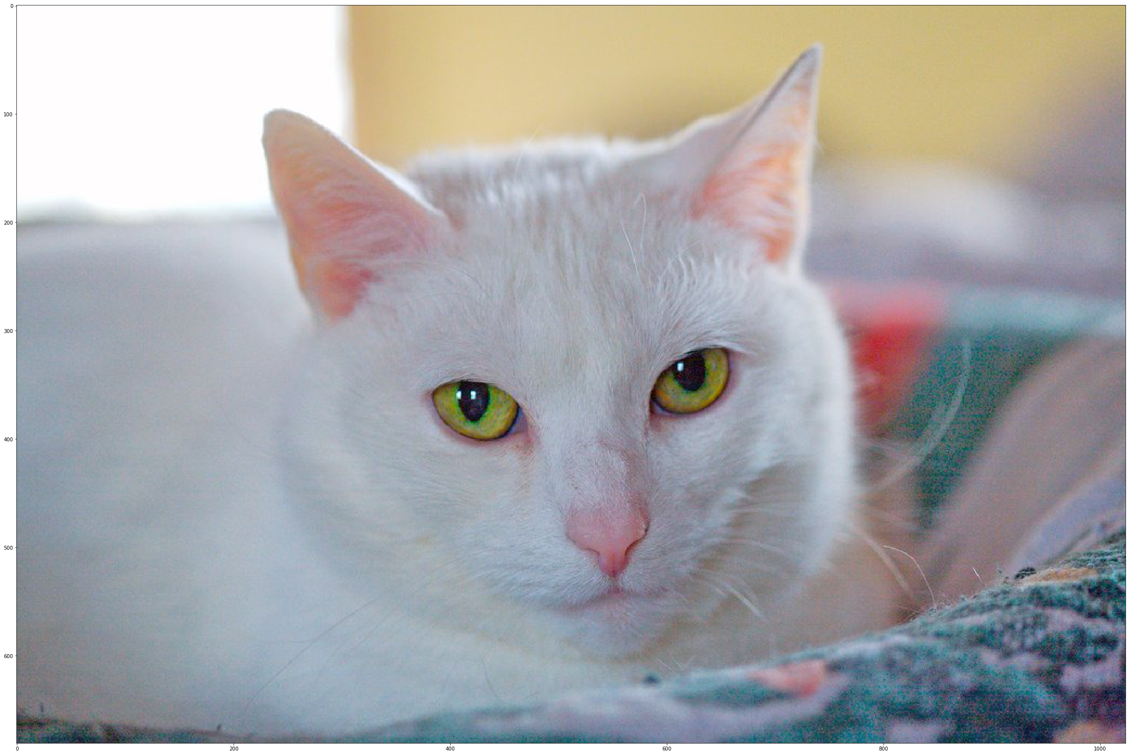
my_image = "my_image.jpg" # change this to the name of your image file
my_label_y = [1] # the true class of your image (1 -> cat, 0 -> non-cat)

fname = "images/" + my_image
image = np.array(ndimage.imread(fname, flatten=False))
my_image = scipy.misc.imresize(image, size=(num_px,num_px)).reshape((num_px*num_px*3,1))
my_image = my_image/255.
my_predicted_image = predict(my_image, my_label_y, parameters)

plt.imshow(image)
print ("y = " + str(np.squeeze(my_predicted_image)) + ", your L-layer model predicts a \"" + classes[int(np.squeeze(my_predicted_image)),].decode("utf-8") +  "\" picture.")

Accuracy: 1.0
y = 1.0, your L-layer model predicts a "cat" picture.

References:

• for auto-reloading external module: http://stackoverflow.com/questions/1907993/autoreload-of-modules-in-ipython