lqsae/pyGenomeTracks

python module to plot beautiful and highly customizable genome browser tracks

pyGenomeTracks

Standalone program and library to plot beautiful genome browser tracks

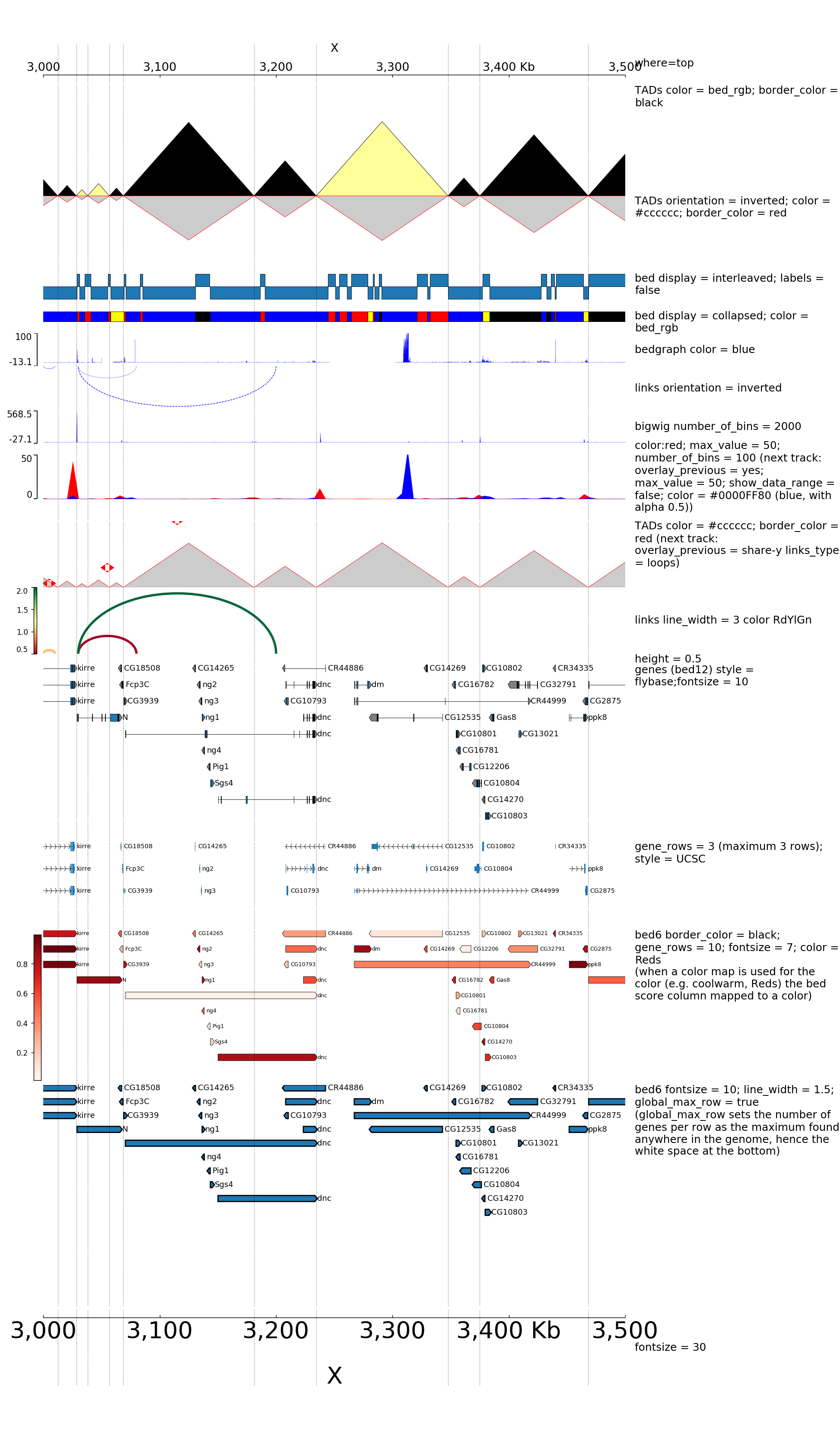
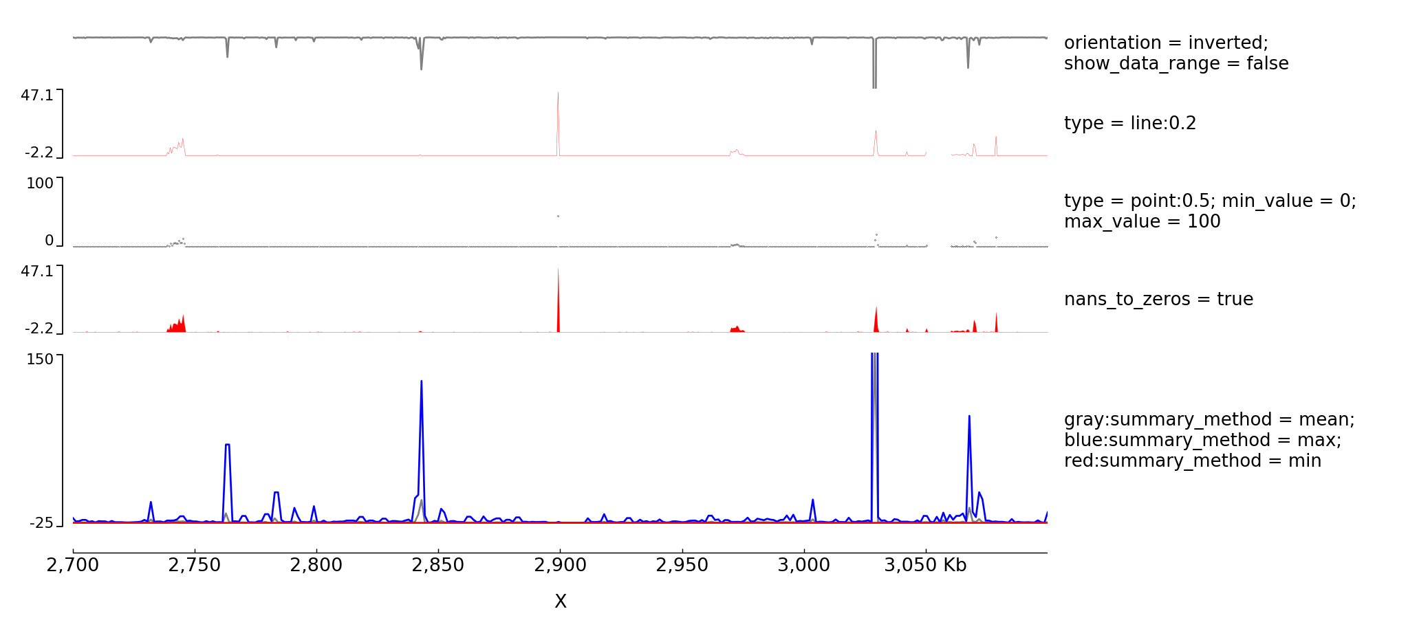
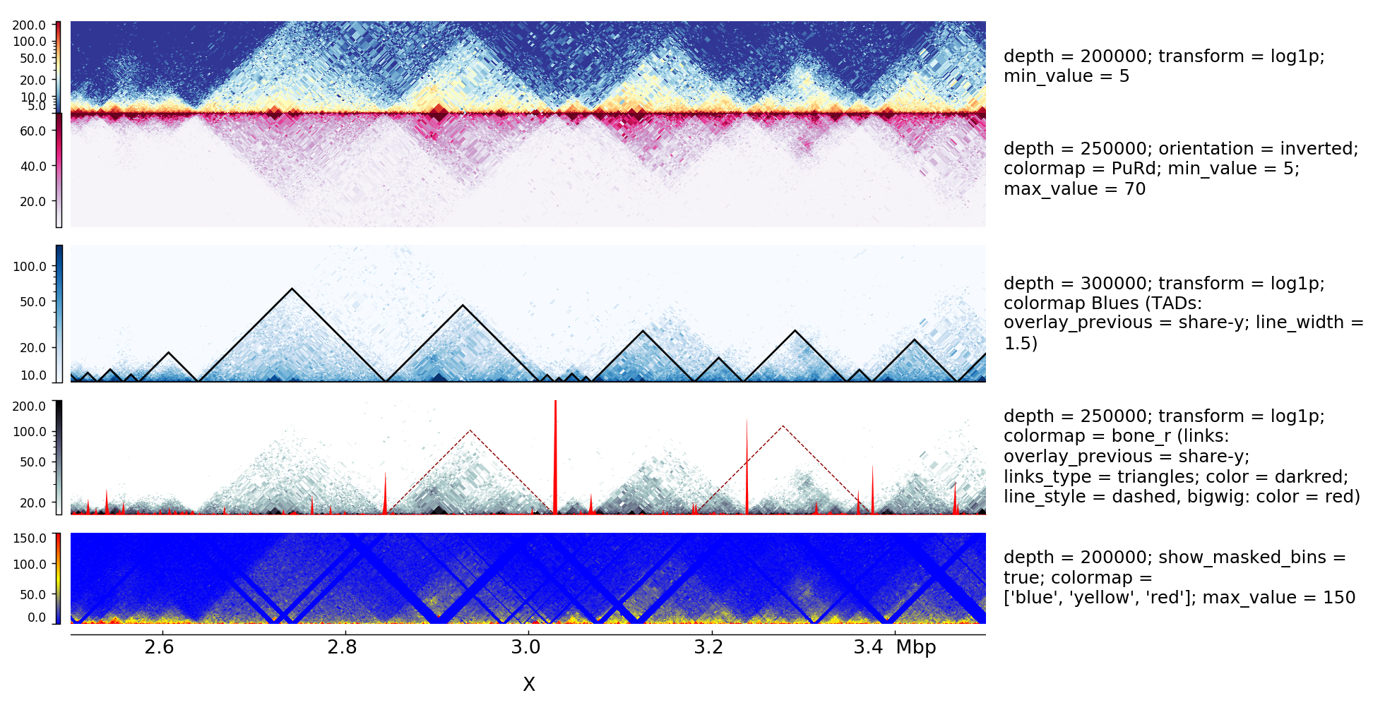
pyGenomeTracks aims to produce high-quality genome browser tracks that are highly customizable. Currently, it is possible to plot:

• bigwig
• bed/gtf (many options)
• bedgraph
• epilogos
• narrow peaks
• links (represented as arcs)
• Hi-C matrices

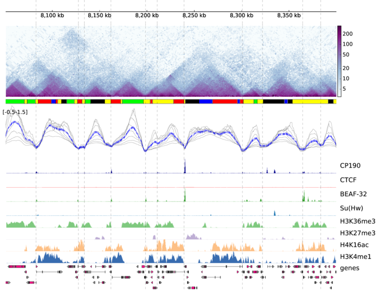
pyGenomeTracks can make plots with or without Hi-C data. The following is an example output of pyGenomeTracks from Ramírez et al. 2017

Table of content

• Installation
• Usage
• Citation
• Examples
• Examples with peaks
• Examples with Hi-C data
• Examples with Epilogos
• Examples with multiple options
• Examples with multiple options for bigwig tracks
• Examples with Hi-C data
• Possible parameters
• Adding new tracks
• External users

Installation

pyGenomeTracks works with python >=3.6.

Currently, the best way to install pyGenomeTracks is with anaconda

$ conda install -c bioconda -c conda-forge pygenometracks

Also, pyGenomeTracks can be installed using pip

$ pip install pyGenomeTracks

If the latest version wants to be installed use:

$ pip install  git+https://github.com/deeptools/pyGenomeTracks.git

Usage

To run pyGenomeTracks a configuration file describing the tracks is required. The easiest way to create this file is using the program make_tracks_file which creates a configuration file with defaults that can be easily changed. The format is:

$ make_tracks_file --trackFiles <file1.bed> <file2.bw> ... -o tracks.ini

make_tracks_file uses the file ending to guess the file type.

Then, a region can be plotted using:

$ pyGenomeTracks --tracks tracks.ini --region chr2:10,000,000-11,000,000 --outFileName nice_image.pdf

The ending --outFileName defines the image format. If .pdf is used, then the resulting image is a pdf. The options are pdf, png and svg.

Description of other possible arguments:

optional arguments:
  -h, --help            show this help message and exit
  --tracks TRACKS       File containing the instructions to plot the tracks.
                        The tracks.ini file can be genarated using the
                        `make_tracks_file` program.
  --region REGION       Region to plot, the format is chr:start-end
  --BED BED             Instead of a region, a file containing the regions to
                        plot, in BED format, can be given. If this is the
                        case, multiple files will be created using a prefix
                        the value of --outFileName
  --width WIDTH         figure width in centimeters
  --height HEIGHT       Figure height in centimeters. If not given, the figure
                        height is computed based on the heights of the tracks.
                        If given, the track height are proportionally scaled
                        to match the desired figure height.
  --title TITLE, -t TITLE
                        Plot title
  --outFileName OUTFILENAME, -out OUTFILENAME
                        File name to save the image, file prefix in case
                        multiple images are stored
  --fontSize FONTSIZE   Font size for the labels of the plot
  --dpi DPI             Resolution for the image in case the ouput is a raster
                        graphics image (e.g png, jpg)
  --trackLabelFraction TRACKLABELFRACTION
                        By default the space dedicated to the track labels is
                        0.05 of the plot width. This fraction can be changed
                        with this parameter if needed.
  --version             show program's version number and exit

Citation

If you use pyGenomeTracks in your analysis, you can cite the following paper :

Fidel Ramírez, Vivek Bhardwaj, Laura Arrigoni, Kin Chung Lam, Björn A. Grüning, José Villaveces, Bianca Habermann, Asifa Akhtar & Thomas Manke. High-resolution TADs reveal DNA sequences underlying genome organization in flies. Nature Communications (2018) doi:10.1038/s41467-017-02525-w

Examples

(These examples are found in the examples/ folder)

A minimal example of a configuration file with a single bigwig track looks like this:

[bigwig file test]
file = bigwig.bw
# height of the track in cm (optional value)
height = 4
title = bigwig
min_value = 0
max_value = 30

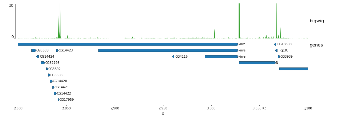
$ pyGenomeTracks --tracks bigwig_track.ini --region X:2,500,000-3,000,000 -o bigwig.png

Now, let's add the genomic location and some genes:

[bigwig file test]
file = bigwig.bw
# height of the track in cm (optional value)
height = 4
title = bigwig
min_value = 0
max_value = 30

[spacer]
# this simply adds an small space between the two tracks.

[genes]
file = genes.bed.gz
height = 7
title = genes
fontsize = 10
file_type = bed
gene_rows = 10

[x-axis]
fontsize=10

$ pyGenomeTracks --tracks bigwig_with_genes.ini --region X:2,800,000-3,100,000 -o bigwig_with_genes.png

Now, we will add some vertical lines across all tracks. The vertical lines should be in a bed format.

[bigwig file test]
file = bigwig.bw
# height of the track in cm (optional value)
height = 4
title = bigwig
min_value = 0
max_value = 30

[spacer]
# this simply adds an small space between the two tracks.

[genes]
file = genes.bed.gz
height = 7
title = genes
fontsize = 10
file_type = bed
gene_rows = 10

[x-axis]
fontsize=10

[vlines]
file = domains.bed
type = vlines

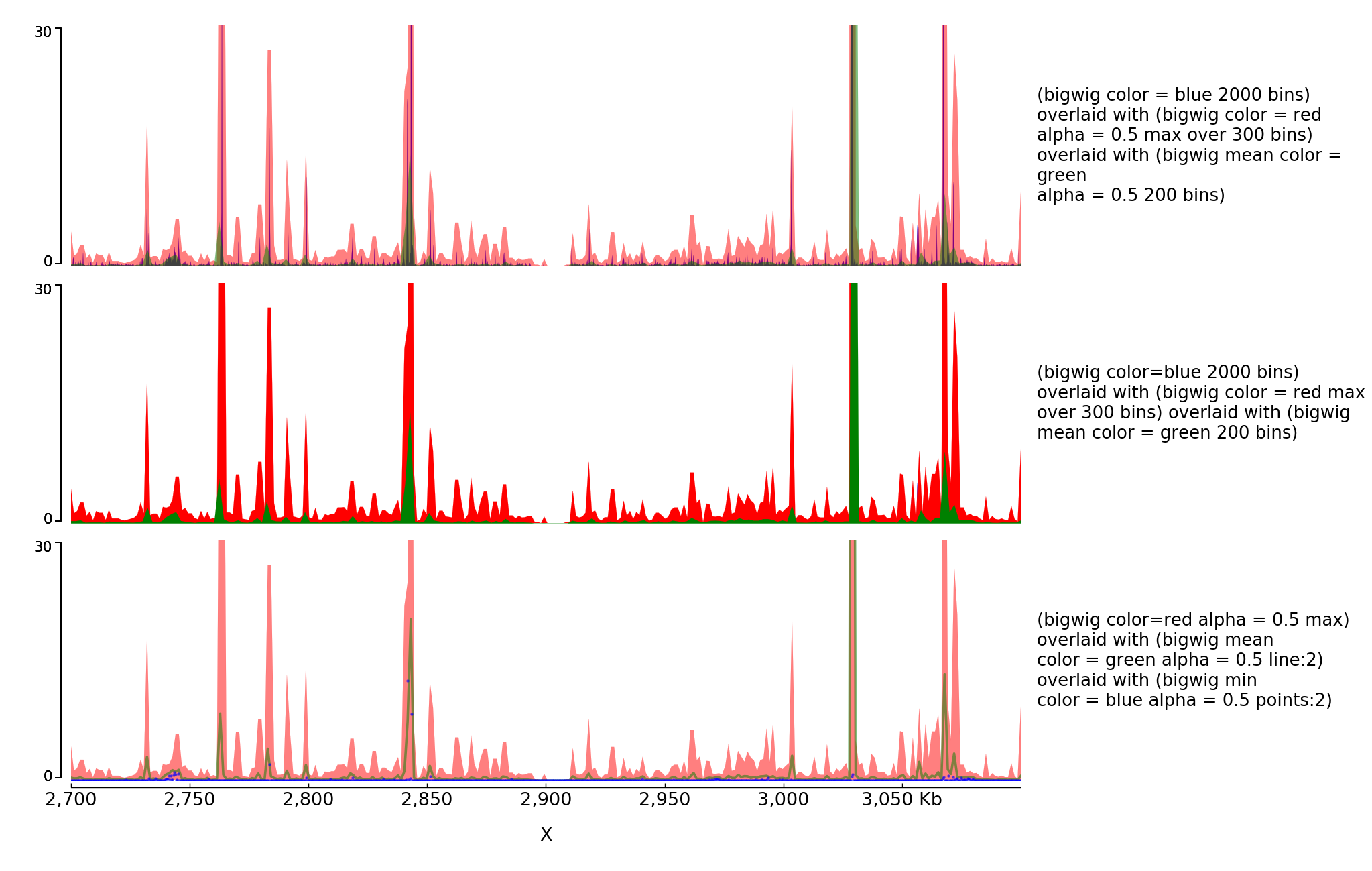
$ pyGenomeTracks --tracks bigwig_with_genes_and_vlines.ini --region X:2,800,000-3,100,000 -o bigwig_with_genes_and_vlines.png

You can also overlay bigwig with or without transparency.

[test bigwig]
file = bigwig2_X_2.5e6_3.5e6.bw
color = blue
height = 7
title = (bigwig color=blue 2000 bins) overlayed with (bigwig mean color=red alpha = 0.5 max over 300 bins) overlayed with (bigwig mean color=red alpha=0.5 200 bins)
number_of_bins = 2000

[test bigwig max]
file = bigwig2_X_2.5e6_3.5e6.bw
color = red
alpha = 0.5
summary_method = max
number_of_bins = 300
overlay_previous = share-y

[test bigwig mean]
file = bigwig2_X_2.5e6_3.5e6.bw
color = green
alpha = 0.5
type = fill
number_of_bins = 200
overlay_previous = share-y

[spacer]


[test bigwig]
file = bigwig2_X_2.5e6_3.5e6.bw
color = blue
height = 7
title = (bigwig color=blue 2000 bins) overlayed with (bigwig mean color=redmax over 300 bins) overlayed with (bigwig mean color=red 200 bins)
number_of_bins = 2000

[test bigwig max]
file = bigwig2_X_2.5e6_3.5e6.bw
color = red
summary_method = max
number_of_bins = 300
overlay_previous = share-y

[test bigwig mean]
file = bigwig2_X_2.5e6_3.5e6.bw
color = green
type = fill
number_of_bins = 200
overlay_previous = share-y


[x-axis]

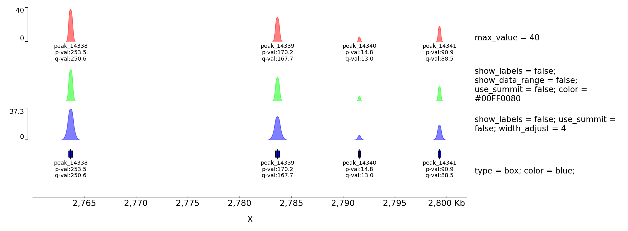
$ pyGenomeTracks --tracks alpha.ini --region X:2700000-3100000 -o master_alpha.png

Examples with peaks

pyGenomeTracks has an option to plot peaks using MACS2 narrowPeak format.

The following is an example of the output in which the peak shape is drawn based on the start, end, summit and height of the peak.

[narrow]
file = test.narrowPeak
height = 4
max_value = 40
title = max_value=40

[narrow 2]
file = test.narrowPeak
height = 2
show_labels = false
show_data_range =  false
color = #00FF0080
use_summit = false
title = show_labels=false; show_data_range=false; use_summit=false;color=#00FF0080
[spacer]

[narrow 3]
file = test.narrowPeak
height = 2
show_labels = false
color = #0000FF80
use_summit = false
width_adjust = 4
title = show_labels=false;width_adjust=3

[spacer]

[narrow 4]
file = test.narrowPeak
height = 3
type = box
color = blue
title = type=box;color=blue;

[x-axis]

Examples with Hi-C data

The following is an example with Hi-C data overlay with topologically associating domains (TADs) and a bigwig file.

[x-axis]
where = top

[hic matrix]
file = hic_data.h5
title = Hi-C data
# depth is the maximum distance plotted in bp. In Hi-C tracks
# the height of the track is calculated based on the depth such
# that the matrix does not look deformed
depth = 300000
transform = log1p
file_type = hic_matrix

[tads]
file = domains.bed
display = triangles
border_color = black
color = none
# the tads are overlay over the hic-matrix
# the share-y options sets the y-axis to be shared
# between the Hi-C matrix and the TADs.
overlay_previous = share-y

[spacer]

[bigwig file test]
file = bigwig.bw
# height of the track in cm (optional value)
height = 4
title = ChIP-seq
min_value = 0
max_value = 30

$ pyGenomeTracks  --tracks hic_track.ini -o hic_track.png --region chrX:2500000-3500000

Examples with Epilogos

pyGenomeTracks can be used to visualize epigenetic states (for example from chromHMM) as epilogos. For more information see: https://epilogos.altiusinstitute.org/

To plot epilogos a qcat file is needed. This file can be crated using the epilogos software (https://github.com/Altius/epilogos).

An example track file for epilogos looks like:

[epilogos]
file = epilog.qcat.bgz
height = 5
title = epilogos

[x-axis]

The color of the bars can be set by using a json file. The structure of the file is like this

{
"categories":{
          "1":["Active TSS","#ff0000"],
          "2":["Flanking Active TSS","#ff4500"],
          "3":["Transcr at gene 5\" and 3\"","#32cd32"],
          "4":["Strong transcription","#008000"]
          }
}

In the following examples the top epilogo has the custom colors and the one below is shown inverted.

[epilogos]
file = epilog.qcat.bgz
height = 5
title = epilogos with custom colors
categories_file = epilog_cats.json

[epilogos inverted]
file = epilog.qcat.bgz
height = 5
title = epilogos inverted
orientation = inverted

[x-axis]

Examples with multiple options

A comprehensive example of pyGenomeTracks can be found as part of our automatic testing. Note, that pyGenome tracks also allows the combination of multiple tracks into one using the parameter: overlay_previous=yes or overlay_previous=share-y. In the second option the y-axis of the tracks that overlays is the same as the track being overlay. Multiple tracks can be overlay together.

The configuration file for this image is here

Examples with multiple options for bigwig tracks

The configuration file for this image is here

Examples with Hi-C data

In these examples is where the overlay tracks are more useful. Notice that any track can be overlay over a Hi-C matrix. Most useful is to overlay TADs or to overlay links using the triangles option that will point in the Hi-C matrix the pixel with the link contact. When overlaying links and TADs is useful to set overlay_previous=share-y such that the two tracks match the positions. This is not required when overlying other type of data like a bigwig file that has a different y-scale.

The configuration file for this image is here

Possible parameters

Here is a table to summarize which are the parameters that can be use for each of the file_type and which is the default value: Empty means this parameter is not used. not set means that by default the parameter is commented.

parameter	x-axis	epilogos	links	domains	bed	narrow_peak	bigwig	bedgraph	bedgraph_matrix	hlines	hic_matrix
where	bottom
fontsize	15			12	12
categories_file		not set
orientation		not set	not set	not set	not set	not set	not set	not set	not set	not set	not set
links_type			arcs
line_width			not set	0.5	0.5					0.5
line_style			solid							solid
color			blue	#1f78b4	#1f78b4	#FF000080	#33a02c	#a6cee3		black
alpha			0.8				1	1		1
max_value			not set	not set	not set	not set	not set	not set	not set	not set	not set
min_value			not set	not set	not set		not set	not set	not set	not set	not set
border_color				black	black
interval_height				100	100
prefered_name				transcript_name	transcript_name
merge_transcripts				false	false
labels					true
style					flybase
display					stacked
max_labels					60
global_max_row					false
gene_rows					not set
arrow_interval					2
arrowhead_included					false
color_utr					grey
height_utr					1
show_data_range						true	true	true	true	true
show_labels						true
use_summit						true
width_adjust						1.5
type						peak	fill	fill	matrix
negative_color							not set	not set
nans_to_zeros							false	false
summary_method							mean	not set
number_of_bins							700	700
use_middle								false
rasterize								false	true		true
pos_score_in_bin									center
plot_horizontal_lines									false
region											not set
depth											100000
show_masked_bins											false
scale_factor											1
transform											no
colormap											RdYlBu_r

Some parameters can take only discrete values.

They are summarized here:

• where:
  • for x-axis: top, bottom
• orientation:
  • for epilogos, links, domains, bed, narrow_peak, bigwig, bedgraph, bedgraph_matrix, hlines, hic_matrix: inverted, not set
• links_type:
  • for links: arcs, triangles, loops
• line_style:
  • for links, hlines: solid, dashed, dotted, dashdot
• style:
  • for bed: flybase, UCSC
• display:
  • for bed: collapsed, triangles, interleaved, stacked
• type:
  • for narrow_peak: peak, box
  • for bedgraph_matrix: matrix, lines
• summary_method:
  • for bigwig: mean, average, max, min, stdev, dev, coverage, cov, sum
  • for bedgraph: mean, average, max, min, stdev, dev, coverage, cov, sum, not set
• pos_score_in_bin:
  • for bedgraph_matrix: center, block
• transform:
  • for hic_matrix: no, log, log1p, -log
• labels:
  • for bed: true, false
• show_data_range:
  • for narrow_peak, bigwig, bedgraph, bedgraph_matrix, hlines: true, false
• plot_horizontal_lines:
  • for bedgraph_matrix: true, false
• use_middle:
  • for bedgraph: true, false
• rasterize:
  • for bedgraph, bedgraph_matrix, hic_matrix: true, false
• global_max_row:
  • for bed: true, false
• show_masked_bins:
  • for hic_matrix: true, false
• show_labels:
  • for narrow_peak: true, false
• use_summit:
  • for narrow_peak: true, false
• merge_transcripts:
  • for domains, bed: true, false
• nans_to_zeros:
  • for bigwig, bedgraph: true, false
• arrowhead_included:
  • for bed: true, false

Adding new tracks

If you are interested in adding new tracks, please see Creating_new_tracks.md.

pyGenomeTracks is used by HiCExporer and HiCBrowser (See e.g. Chorogenome navigator which is made with HiCBrowser)

External users

• CoolBox is an interactive genomic data explorer for Jupyter Notebooks
• Galaxy integration offers a graphical user-interface to create PGT plots. It is also possible to include PGT into workflows and automatic pipelines.