openTSNE

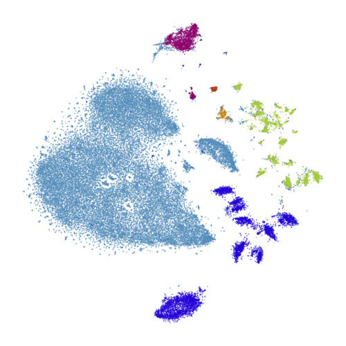
openTSNE is a modular Python implementation of t-Distributed Stochasitc Neighbor Embedding (t-SNE) [1], a popular dimensionality-reduction algorithm for visualizing high-dimensional data sets. openTSNE incorporates the latest improvements to the t-SNE algorithm, including the ability to add new data points to existing embeddings [2], massive speed improvements [3] [4], enabling t-SNE to scale to millions of data points and various tricks to improve global alignment of the resulting visualizations [5].

Macosko 2015 mouse retina t-SNE embedding

A visualization of 44,808 single cell transcriptomes obtained from the mouse retina [6] embedded using the multiscale kernel trick to better preserve the global aligment of the clusters.

Documentation
User Guide and Tutorial
Examples: basic, advanced, preserving global alignment, embedding large data sets
Speed benchmarks

Installation

openTSNE requires Python 3.6 or higher in order to run.

Conda

openTSNE can be easily installed from conda-forge with

conda install --channel conda-forge opentsne

Conda package

PyPi

openTSNE is also available through pip and can be installed with

pip install opentsne

PyPi package

Installing from source

If you wish to install openTSNE from source, please run

python setup.py install

in the root directory to install the appropriate dependencies and compile the necessary binary files.

Please note that openTSNE requires a C/C++ compiler to be available on the system. Additionally, numpy must be pre-installed in the active environment.

In order for openTSNE to utilize multiple threads, the C/C++ compiler must support OpenMP. In practice, almost all compilers implement this with the exception of older version of clang on OSX systems.

To squeeze the most out of openTSNE, you may also consider installing FFTW3 prior to installation. FFTW3 implements the Fast Fourier Transform, which is heavily used in openTSNE. If FFTW3 is not available, openTSNE will use numpy’s implementation of the FFT, which is slightly slower than FFTW. The difference is only noticeable with large data sets containing millions of data points.

A hello world example

Getting started with openTSNE is very simple. First, we'll load up some data using scikit-learn

from sklearn import datasets

iris = datasets.load_iris()
x, y = iris["data"], iris["target"]

then, we'll import and run

from openTSNE import TSNE

embedding = TSNE().fit(x)

Citation

If you make use of openTSNE for your work we would appreciate it if you would cite the paper

@article {Poli{\v c}ar731877,
    author = {Poli{\v c}ar, Pavlin G. and Stra{\v z}ar, Martin and Zupan, Bla{\v z}},
    title = {openTSNE: a modular Python library for t-SNE dimensionality reduction and embedding},
    year = {2019},
    doi = {10.1101/731877},
    publisher = {Cold Spring Harbor Laboratory},
    URL = {https://www.biorxiv.org/content/early/2019/08/13/731877},
    eprint = {https://www.biorxiv.org/content/early/2019/08/13/731877.full.pdf},
    journal = {bioRxiv}
}

openTSNE implements two efficient algorithms for t-SNE. Please consider citing the original authors of the algorithm that you use. If you use FIt-SNE (default), then the citation is [4] below, but if you use Barnes-Hut the citation is [3].

References

[1]	Van Der Maaten, Laurens, and Hinton, Geoffrey. “Visualizing data using t-SNE.” Journal of Machine Learning Research 9.Nov (2008): 2579-2605.

[2]	Poličar, Pavlin G., Martin Stražar, and Blaž Zupan. “Embedding to Reference t-SNE Space Addresses Batch Effects in Single-Cell Classification.” BioRxiv (2019): 671404.

[3]	(1, 2) Van Der Maaten, Laurens. “Accelerating t-SNE using tree-based algorithms.” Journal of Machine Learning Research 15.1 (2014): 3221-3245.

[4]	(1, 2) Linderman, George C., et al. "Fast interpolation-based t-SNE for improved visualization of single-cell RNA-seq data." Nature Methods 16.3 (2019): 243.

[5]	Kobak, Dmitry, and Berens, Philipp. “The art of using t-SNE for single-cell transcriptomics.” Nature Communications 10, 5416 (2019).

[6]	Macosko, Evan Z., et al. “Highly parallel genome-wide expression profiling of individual cells using nanoliter droplets.” Cell 161.5 (2015): 1202-1214.

lucaspedroni/openTSNE