In this lesson, we'll learn about the most popular and widely-used clustering algorithm, K-means clustering.
You will be able to:
- Compare the different approaches to clustering networks
- Explain the steps behind the K-means clustering algorithm
- Perform k-means clustering in scikit-learn
- Explain how clusters are evaluated
- Define an "elbow plot" and how to interpret it
Clustering techniques are among the most popular unsupervised machine learning algorithms. The main idea behind clustering is that you want to group objects into similar classes, in a way that:
- intra-class similarity is high (similarity amongst members of the same group is high)
- inter-class similarity is low (similarity of different groups is low)
What does similarity mean? You should be thinking of it in terms of distance, just like we did with the k-nearest-neighbors algorithm. The closer two points are, the more similar they are. It is useful to make a distinction between hierarchical and nonhierarchical clustering algorithms:
-
In cluster analysis, an agglomerative hierarchical algorithm starts with n clusters (where n is the number of observations, so each observation is a cluster), then combines the two most similar clusters, combines the next two most similar clusters, and so on. A divisive hierarchical algorithm does the exact opposite, going from 1 to n clusters.
-
A nonhierarchical algorithm chooses k initial clusters and reassigns observations until no improvement can be obtained. How initial clusters and reassignments are done depends on the specific type of algorithm.
An essential understanding when using clustering methods is that you are basically trying to group data points together without knowing what the actual cluster/classes are. This is also the main distinction between clustering and classification (which is a supervised learning method). This is why technically, you also don't know how many clusters you're looking for.
K-means clustering is the most well-known clustering technique, and it belongs to the class of non-hierarchical clustering methods. When performing k-means clustering, you're essentially trying to find
The k-means clustering algorithm is an iterative algorithm that reaches for a pre-determined number of clusters within an unlabeled dataset, and basically works as follows:
- Select
$k$ initial seeds - Assign each observation to the cluster to which it is "closest"
- Recompute the cluster centroids
- Reassign the observations to one of the clusters according to some rule
- Stop if there is no reallocation
Two assumptions are of main importance for the k-means clustering algorithm:
- To compute the "cluster center", you calculate the (arithmetic) mean of all the points belonging to the cluster. Each cluster center is recalculated in the beginning of each new iteration
- After the cluster center has been recalculated, if a given point is now closer to a different cluster center than the center of its current cluster, then that point is reassigned to the clostest center
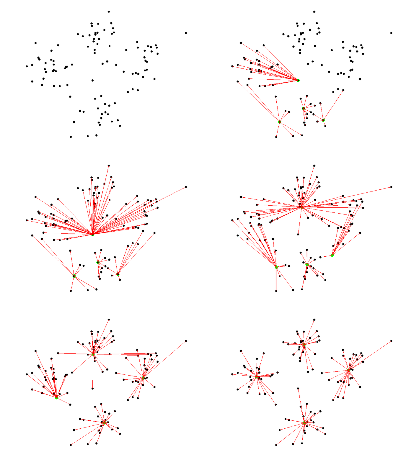
In the animation below, the green dots are the centroids. Notice how they are randomly assigned at the beginning, and shift with each iteration as they are recalculated to match the center of the points assigned to their cluster. The clustering ends when the centroids find a position in which points are no longer reassigned, meaning that the centroids no longer need to move.
Implementing k-means clustering with scikit-learn is quite simple because the API mirrors the same functionality that we've seen before. The same preprocessing steps used for supervised learning methods are required -- missing values must be dealt with and all data must be in numerical format (meaning that non-numerical columns must be dropped or one-hot encoded).
from sklearn.cluster import KMeans

# Set number of clusters at initialization time
k_means = KMeans(n_clusters=3)

# Run the clustering algorithm
k_means.fit(some_df)

# Generate cluster index values for each row
cluster_assignments = k_means.predict(some_df)

# Cluster predictions for each point are also stored in k_means.labels_Running K-means on a dataset is easy enough, but how do we know if we have the best value for
The variance ratio is a ratio of the variance of the points within a cluster, to the variance of a point to points in other clusters. Intuitively, we can understand that we want intra-cluster variance to be low (suggesting that the clusters are tightly knit), and inter-cluster variance to be high (suggesting that there is little to no ambiguity about which cluster the points belong to).
We can easily calculate the variance ratio by importing a function from scikit-learn to calculate it for us, as shown below. To use this metric, we just need to pass in the points themselves, and the predicted labels given to each point by the clustering algorithm. The higher the score, the better the fit.
# This code builds on the previous example
from sklearn.metrics import calinski_harabasz_score

# Note that we could also pass in k_means.labels_ instead of cluster_assignments
print(calinski_harabasz_score(some_df, cluster_assignments))
There are other metrics that can also be used to evaluate the fitness, such as Silhouette Score. No one metric is best -- they all have slightly different strengths and weaknesses depending on the given dataset and goals. Because of this, it's generally accepted that it's best to pick one metric and stick to it.
Now that we have a way to evaluate how well our clusters fit the dataset, we can use this to find the optimal value for
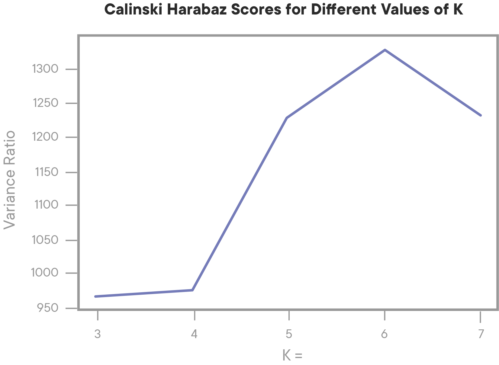
We can then visualize the scores using an Elbow Plot:
An elbow plot is a general term for plots like this where we can easily see where we hit a point of diminishing returns. In the plot above, we can see that performance peaks at k=6, and then begins to drop off. That tells us that our data most likely has 6 naturally occurring clusters in our data.
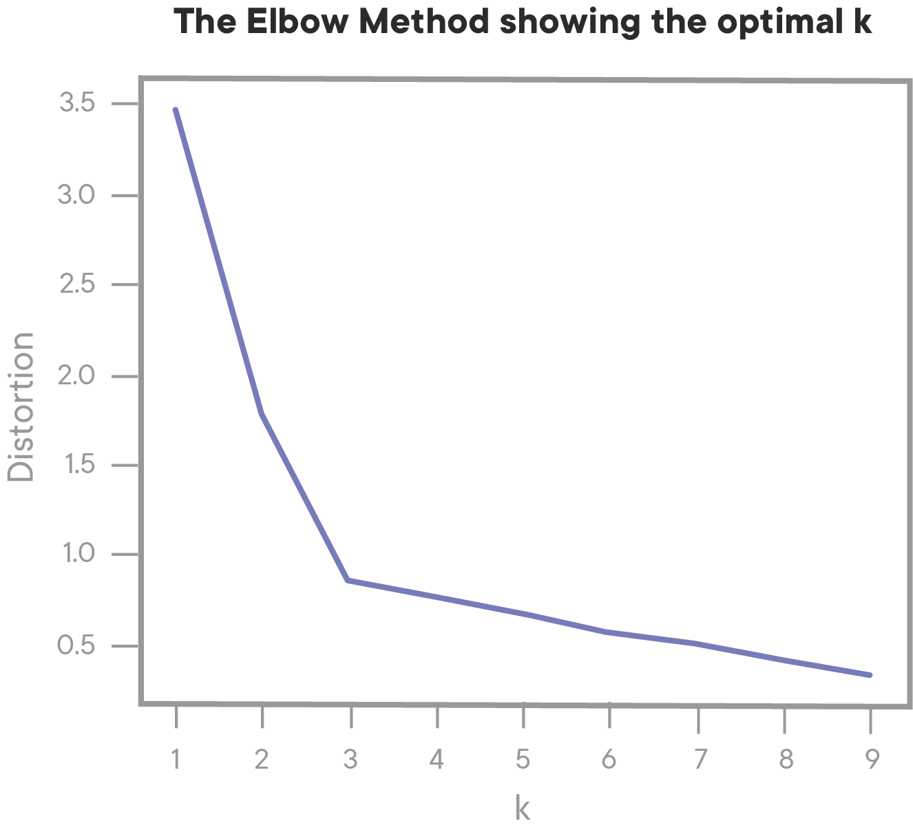
Elbow plots aren't exclusively used with variance ratios -- it's also quite common to calculate something like distortion (another clustering metric), which will result in a graph with a negative as opposed to a positive slope.
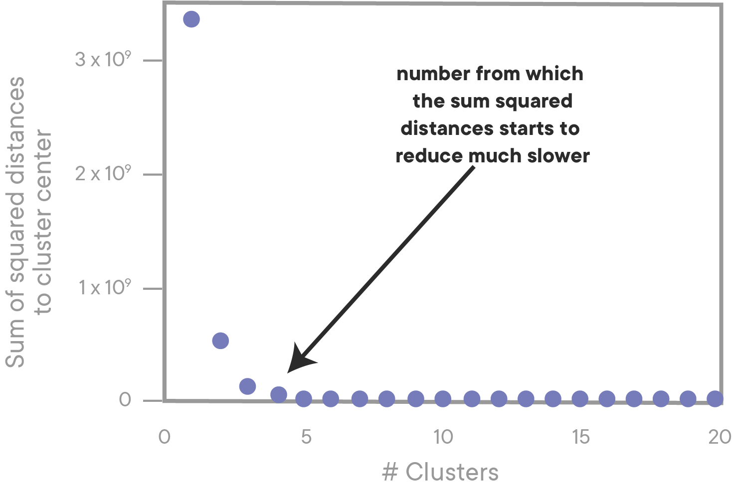
A note on elbow plots: higher scores aren't always better. Higher values of
In the example above, although k=20 technically scores better than k=4, we choose k=4 because it is the Elbow on the graph. After the elbow, the metric we're trying to optimize for gets better at a much slower rate. Dealing with 20 clusters, when the fit is only slightly better, isn't worth it -- it's better to treat our data as having only 4 clusters, because that is the simplest overall model that provides the most value with the least complexity!
In this lesson, we learned about different kinds of clustering and explored how the k-means clustering algorithm works. We also learned about how we can quantify the performance of a clustering algorithm using metrics such as variance ratios, and how we can use these metrics to find the optimal value for


