geo-HPC course

Parallel CPU and GPU high-performance computing course

This short course aims at providing an interactive and applied approach in an hands-on format to parallel and high-performance computing in Julia. This short course covers trendy areas in modern geocomputing. Seeking at solutions of differential equations requires efficient numerical schemes optimally leveraging modern hardware. These solvers permit to resolve scientific problems that where technically not possible a decade ago.

The goal of this short course is to offer an interactive and tutorial-like hands-on to solve systems of differential equations in parallel on many-core hardware accelerators such as GPUs using the Julia language. Julia combines high-level language simplicity to low-level language performance. The resulting codes and applications are fast, short and readable [1, 2, 3].

The iterative algorithms can be converted into efficient linear and non-linear solvers relying on a second order Richardson type of iterations strategy [4].

Content

Objectives
Pre-requisite
Material
Getting started
Course outline
Advanced start
Extras
Further reading

Objectives

We will design and implement an iterative numerical algorithm that resolves (non-linear) diffusion in 2D for two applications:

The diffusion of heat:

dT/dt	= 1/ρCp*(-dqx/dx -dqy/dy)
qx     	= -λ*dT/dx
qy     	= -λ*dT/dy

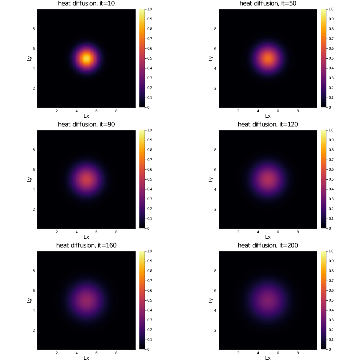
For an initial Gaussian distribution, the heat diffusion code produces following output:

The non-linear diffusion of ice topography (simplified shallow-ice):

dH/dt	= -dqx/dx -dqy/dy + b
qx     	= -H^n*dH/dx
qy     	= -H^n*dH/dy

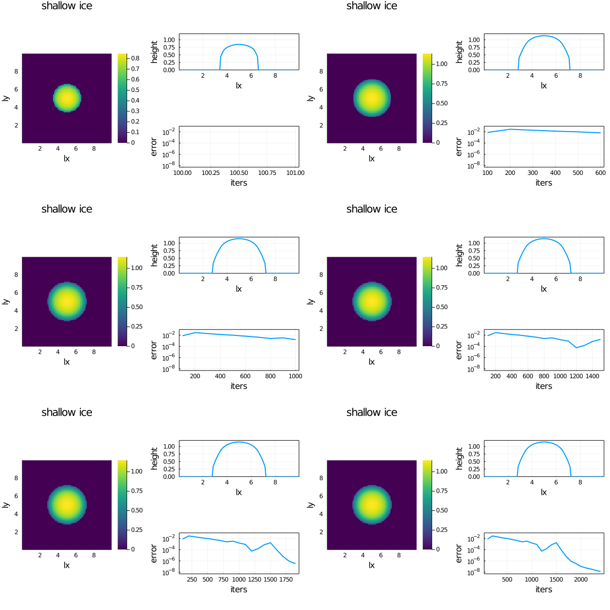
For an initial Gaussian distribution of ice and a circular and centred source/sink term, the simplified shallow-ice code produces following output while reaching a steady state:

These two examples will enable to address the technical objectives of this course (3 parts).

Technical objectives of this course (3 parts)

Part 1 | We will use (1) as playground to address:

vectorised plain Julia implementation CPU (idem as python, Matlab, Octave)
vectorised versus loop versions on CPU
"kernel"-style loops and multi-threading multi-core CPU
vectorised plain Julia with GPU backend (similar to abstract GPU functions for e.g. python, Matlab)
explicit "kernel"-style GPU (Julia's power: C CUDA low-level handles)
enabling single/multi-XPU (both multi-core CPU and GPU) using ParallelStencil.jl

Part 2 | We will use (2) as playground to address:

explicit time stepping
transient, steady-state solutions
explicit vs implicit solutions

Part 3 | We will use (1) and (2) to address:

distributed memory parallelisation ("fake" and "real" parallelisation)
local and global domain, internal and global boundaries, initial condition, boundary update, synchronisation
visualisation and I/O
message passing interface (MPI), MPI + GPU (CUDA-aware MPI)
communication/computation overlap (hide communication)
using ImplicitGlobalGrid.jl for high-level implementation along with ParallelStencil.jl

Pre-requisite

The hands-on format prioritises the learning-by-doing thus not much preliminary knowledge is required. Basic programming skills won't hurt though. The course will build upon the use of the Julia programming language.

Performance metric to compare the various code implementations

Majority of stencil based codes as in this course are memory bounded, meaning the limiting factor in performance is the rate at which memory is transferred from and back between the memory and the arithmetic units. The maximal rate at which the memory transfers occur is the memory copy rate, in the order of 50 GB/s for CPUs and about 1 TB/s for modern GPUs. The effective memory throughput metric (T_eff) measures how good an iterative stencil-based algorithm performs in terms of memory throughput, to be compared to the memory copy rate. The T_eff formula reads: T_eff = (nIO/1e9*nxy*PRECIS)/(time_s/nt), where nIO is the number of read/write operations (2 for an update rule), nxy is the numerical grid resolution, PRECIS is the arithmetic precision (8 or 4 bytes per number), time_s is the execution time in second to perform nt iterations [1].

Programming in Julia

On the CPU, multi-threading is made accessible via Base.Threads and the environment variable JULIA_NUM_THREADS can be used to define the number of cores to use on the CPU, e.g. export JULIA_NUM_THREADS=2 to enable 2 threads (2 CPU cores). The CUDA.jl module permits to launch compute kernels on Nvidia GPUs within Julia. JuliaGPU provides further reading and introductory material about GPU ecosystem within Julia.

Material

The course material contains some ready-to-run example scripts, draft tmp scripts to be complete as tasks during the course and their corresponding solution scripts.

example scripts | The active working directory for the course will be scripts, that contains the example scripts and the tmp scripts to work on.
solution scripts | All tmp scripts have their corresponding solution scripts located in solutions

Getting started

If it applies, follow the instructions provided on the course's private channel.

Julia quick start

In general, clone this repo (or download it otherwise) to run the example scripts and access the draft scripts to be completed during the course. Solutions or "cheat-sheets" can be found in the solutions folder. The examples rely on 3 main Julia modules, Plots.jl (and PyPlot.jl) and CUDA.jl. The XPU examples require ParallelStencil.jl to be installed. The MPI examples require MPI.jl to be installed. The multi-XPU scripts require ImplicitGlobalGrid.jl to be installed.

There are two ways of executing a Julia script, from the Julia command window known as the Julia REPL, or from the terminal shell directly. The MPI and multi-XPU examples need to be executed from the terminal shell.

To run Julia interactively, start Julia from the shell (or Terminal). Go to the geo-hpc-course folder. Then start Julia appending the --project flag to gain access to the required modules:

$ cd <path-to>/geo-hpc-course/
$ julia --project

Then, in the Julia REPL, you can execute the script as following:

julia> include("<my_script>.jl")

💡 Note that typing ; in the Julia REPL permits you to execute shell commands (like cd ..).

For optimal performance (like measuring T_eff) and for running Julia MPI, run Julia as executable from the shell directly, using the optimisation flag -O3 and disabling bound checking --check-bounds=no as following:

$ julia --project -O3 --check-bounds=no <my_script>.jl

Note that interactive plotting may fail then.

Set the default viz = false flag to true if you want to plot output in all codes beyond step 2.

Running Julia MPI

This section is about launching a Julia MPI script. For MPI.jl install notes, refer to the Advanced start - Julia MPI section and the MPI.jl doc. In the proposed approach, each MPI process will handle one CPU thread. In the MPI GPU case (multi-GPUs), each MPI process handles one GPU.

Assuming a working Julia MPI installation, a Julia MPI program can be launched using the Julia MPI wrapper mpiexecjl (located in ~/.julia/bin).

Running the Julia MPI hello_mpi.jl script on 4 processes can be achieved following:

$ mpiexecjl -n 4 julia --project scripts/hello_mpi.jl
$ Hello world, I am 0 of 3
$ Hello world, I am 1 of 3
$ Hello world, I am 2 of 3
$ Hello world, I am 3 of 3

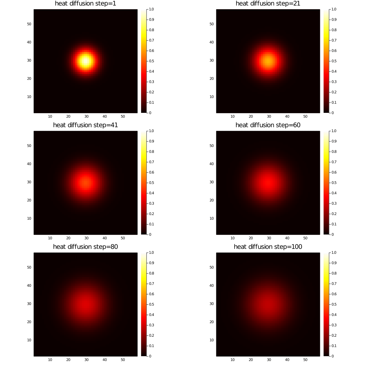
The 2D Julia MPI diffusion script heat_2D_mpi.jl executed on 4 MPI processes (global grid: 2x2) produces the following output (see Extras for infos about the gif-making scripts).

Note: The presented concise Julia MPI scripts are inspired from this 2D python script.

Advanced documentation on running the multi-XPU codes can be found in the ParallelStencil.jl module documentation.

Course outline

During the course, we will go through the following steps:

Intro part 1
TODO Finalise the 1D heat diffusion code heat_1D_tmp.jl, implementing the equations from Objectives 1.
See how the diffusion looks like in 2D heat_2D.jl.
TODO Finalise the 2D loop version of the heat code heat_2D_loop_tmp.jl.
TODO Import the flux and T loop calculations in the heat code using external "kernel"-like compute functions heat_2D_loop_fun_tmp.jl.
See how the function-based loop version (5.) can be further extended to checking bounds with if statement in the ix and iy loops, including "loop-fusion" for the flux computations heat_2D_loop_fun_gpustyle.jl.
See how one can simply use the GPU to perform the 2D heat diffusion calculations heat_2D_gpu.jl.
TODO The performance "magic"; update the script heat_2D_gpu_fun_tmp.jl based on previous knowledge and step (5.).
See how steps 5., 6. and 7. can be combined into a single code using ParallelStencil.jl in heat_2D_xpu.jl
Discussion on CPU vs GPU architectures and performance evaluation (T_eff). Q&A.

Intro part 2
TODO Based on your acquired experience, finalise the sia_2D_tmp.jl script to convert the heat diffusion T into an ice cap thickness H evolution over time.
TODO Modify the the script from (12.) to have an implicit solver while reaching a steady-state solution.
TODO (NEW!) You demystified GPU computing with completing step 9. Update now the script sia_2D_xpu_tmp.jl to have an XPU (CPU or GPU) code ready!
Discussion about pseudo-transient solvers, damping and convergence. Q&A.

Intro part 3 (NEW!)
TODO Finalise the 1D heat diffusion code heat_1D_2procs_tmp.jl, splitting the calculation of temperature evolution on one left and one right domain. This "fake-parallelisation" requires left and right temperature arrays, TL and TR, respectively.
TODO Generalise the "fake-parallel" approach on 2 processes to n processes by modifying the code heat_1D_nprocs_tmp.jl, taking care of implementing the initial condition, heat diffusion physics and the boundary update.
The script hello_mpi.jl shows a "Hello World" example implementing MPI.jl. Use this script to test your MPI.jl install (see the Running Julia MPI section for more infos on installing and running Julia MPI).
Discover a concise MPI 1D heat diffusion example heat_1D_mpi.jl. Learn about the minimal requirements to initialise a Cartesian MPI topology and how to code the boundary update functions (here using blocking messages). Use the vizme1D_mpi.jl script to visualise the results (each MPI process saving it's local output).
TODO Yay, you have your MPI 1D Julia script running! Finalise the MPI 2D heat diffusion script heat_2D_mpi_tmp.jl to solve the 2D diffusion equation using MPI. Use the vizme2D_mpi.jl script to visualise the results (each MPI process saving it's local output).
Now that you demystified distributed memory parallelisation, see how using ImplicitGlobalGrid.jl along with ParallelStencil.jl leads to concise and efficient distributed memory parallelisation on multiple XPUs in 2D heat_2D_multixpu.jl. Also, take a closer look at the @hide_communication feature. Further infos can be found here.
TODO Instrument the 2D shallow ice code sia_2D_xpu.jl (task 14.) to enable distributed memory parallelisation using ImplicitGlobalGrid.jl along with ParallelStencil.jl.

💡 Use sia_2D_xpu.jl for a quick start, and sia_2D_multixpu.jl for a solution.

Yay, you made it - you demystified running Julia codes in parallel on multi-XPU :-) Q&A.

Advanced start

Steps already done on the GPU server you are running on (CentOS 8 linux)

Julia

Starting in the shell:

$ wget https://julialang-s3.julialang.org/bin/linux/x64/1.6/julia-1.6.2-linux-x86_64.tar.gz
$ tar -xzf julia-1.6.2-linux-x86_64.tar.gz
$ vim ~/.bashrc # Add the line: PATH=~/julia-1.6.2/bin/:$PATH
$ cd <path-to>/geo-hpc-course/
$ julia --project

Once Julia launched, enter the package mode ] and instantiate the project. This will download all the project's dependencies and install them:

julia> ]

(geo-hpc-course) pkg> instantiate

julia>

If your GPU system contains more than one GPU, you can add following at the beginning of each gpu named code to target a specific device identified by its unique ID (default being 0):

GPU_ID = ID
CUDA.device!(GPU_ID)

Julia MPI

The following steps permit you to install MPI.jl on your machine:

Add MPI.jl:

(project) pkg> add MPI

julia> using MPI
[ Info: Precompiling MPI [da04e1cc-30fd-572f-bb4f-1f8673147195]

julia> MPI.install_mpiexecjl()
[ Info: Installing `mpiexecjl` to `HOME/.julia/bin`...
[ Info: Done!

Then, one should add HOME/.julia/bin to PATH in order to launch the Julia MPI wrapper mpiexecjl.
Running the Julia MPI code on 4 processes:

$ HOME/.julia/bin/mpiexecjl -n 4 julia --project scripts/hello_mpi.jl

💡 Note: On MacOS, there seems to be an issue (JuliaParallel/MPI.jl#407). To fix it, define following ENV variable:

$ export MPICH_INTERFACE_HOSTNAME=localhost

and add -host localhost to the execution script:

$ HOME/.julia/bin/mpiexecjl -n 4 -host localhost julia --project scripts/hello_mpi.jl

Extras

Julia supports UTF-8 (Unicode) characters. Also, the plotting package Plots.jl permits to create gif animation out-of-the-box. The /extras/heat_2D_gif_unicode.jl exemplifies these two fun capabilities.

The code /extras/sia_2D_ss_gif.jl uses the out-of-the-box gif-making capabilities to produce the SIA non-linear diffusion gif.

The code /extras/heat_2D_mpi_gif.jl produces time-dependent output to be visualised as a gif using the /extras/vizme2D_mpi_gif.jl script.

💡 Note: On Linux machines, emoji keyboard may need to be installed in order to display the Unicode emoticons.

$ sudo dnf install google-noto-emoji-color-fonts.noarch

luraess/geo-hpc-course