BERTopic is a topic modeling technique that leverages BERT embeddings and c-TF-IDF to create dense clusters allowing for easily interpretable topics whilst keeping important words in the topic descriptions.
Corresponding medium post can be found here.
- About the Project
- Getting Started
2.1. Installation
2.2. Basic Usage
2.3. Custom Embeddings
2.4. Visualize Topic Probabilities
2.5. Overview - Algorithm
3.1. Sentence Transformer
3.2. UMAP + HDBSCAN
3.3. c-TF-IDF - Google Colaboratory
The initial purpose of this project was to generalize Top2Vec such that it could be used with state-of-art pre-trained transformer models. However, this proved difficult due to the different natures of Doc2Vec and transformer models. Instead, I decided to come up with a different algorithm that could use BERT and 🤗 transformers embeddings. The results is BERTopic, an algorithm for generating topics using state-of-the-art embeddings.
PyTorch 1.2.0 or higher is recommended. If the install below gives an error, please install pytorch first here.
Installation can be done using pypi:
pip install bertopic
Below is an example of how to use the model. The example uses the 20 newsgroups dataset.
from bertopic import BERTopic
from sklearn.datasets import fetch_20newsgroups

docs = fetch_20newsgroups(subset='all')['data']

model = BERTopic("distilbert-base-nli-mean-tokens", verbose=True)
topics, probabilities = model.fit_transform(docs)
The resulting topics can be accessed through model.get_topic(topic):
>>> model.get_topic(9)
[('game', 0.005251396890032802),
 ('team', 0.00482651185323754),
 ('hockey', 0.004335032060690186),
 ('players', 0.0034782716706978963),
 ('games', 0.0032873248432630227),
 ('season', 0.003218987432255393),
 ('play', 0.0031855141725669637),
 ('year', 0.002962343114817677),
 ('nhl', 0.0029577648449943144),
 ('baseball', 0.0029245163154193524)]
You can find an overview of all models currently in BERTopic here and here.
If you use BERTopic as shown above, then you are forced to use sentence-transformers as the main
package for which to create embeddings. However, you might have your own model or package that
you believe is better suited for representing documents.
Fortunately, for those that want to use their own embeddings there is an option in BERTopic.
For this example I will still be using sentence-transformers but the general principle holds:
from bertopic import BERTopic
from sklearn.datasets import fetch_20newsgroups
from sentence_transformers import SentenceTransformer

# Prepare embeddings
docs = fetch_20newsgroups(subset='all')['data']
sentence_model = SentenceTransformer("distilbert-base-nli-mean-tokens")
embeddings = sentence_model.encode(docs, show_progress_bar=False)

# Create topic model
model = BERTopic(verbose=True)
topics = model.fit_transform(docs, embeddings)
Due to the stochastisch nature of UMAP, the results from BERTopic might differ even if you run the same code multiple times. Using your own embeddings allows you to try out BERTopic several times until you find the topics that suit you best. You only need to generate the embeddings itself once and run BERTopic several times with different parameters.
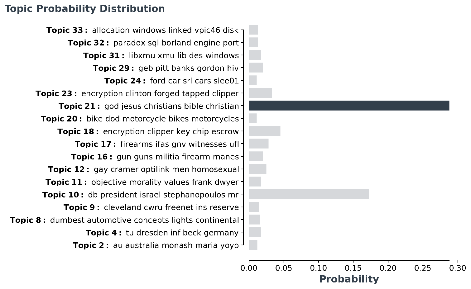
The variable probabilities that is returned from transform() or fit_transform() can
be used to understand how confident BERTopic is that certain topics can be found in a document.
To visualize the distributions, we simply call:
# Make sure to input the probabilities of a single document!
model.visualize_distribution(probabilities[0])NOTE: The distribution of the probabilities does not give an indication to the distribution of the frequencies of topics across a document. It merely shows how confident BERTopic is that certain topics can be found in a document.
| Methods | Code | Returns |
|---|---|---|
| Access single topic | model.get_topic(12) |
Tuple[Word, Score] |
| Access all topics | model.get_topics() |
List[Tuple[Word, Score]] |
| Get single topic freq | model.get_topic_freq(12) |
int |
| Get all topic freq | model.get_topics_freq() |
DataFrame |
| Fit the model | model.fit(docs]) |
- |
| Fit the model and predict documents | model.fit_transform(docs]) |
List[int], List[float] |
| Predict new documents | model.transform([new_doc]) |
List[int], List[float] |
| Visualize Topic Probability Distribution | model.visualize_distribution(probabilities) |
Matplotlib.Figure |
| Save model | model.save("my_model") |
- |
| Load model | BERTopic.load("my_model") |
- |
NOTE: The embeddings itself are not preserved in the model as they are only vital for creating the clusters.
Therefore, it is advised to only use fit and then transform if you are looking to generalize the model to new documents.
For existing documents, it is best to use fit_transform directly as it only needs to generate the document
embeddings once.
Back to ToC
The algorithm contains, roughly, 3 stages:
- Extract document embeddings with Sentence Transformers
- Cluster document embeddings to create groups of similar documents with UMAP and HDBSCAN
- Extract and reduce topics with c-TF-IDF
We start by creating document embeddings from a set of documents using sentence-transformer. These models are pre-trained for many language and are great for creating either document- or sentence-embeddings.
If you have long documents, I would advise you to split up your documents into paragraphs or sentences as a BERT-based
model in sentence-transformer typically has a token limit.
Next, in order to cluster the documents using a clustering algorithm such as HDBSCAN we first need to reduce its dimensionality as HDBCAN is prone to the curse of dimensionality.
Thus, we first lower dimensionality with UMAP as it preserves local structure well after which we can use HDBSCAN to cluster similar documents.
What we want to know from the clusters that we generated, is what makes one cluster, based on their content, different from another? To solve this, we can modify TF-IDF such that it allows for interesting words per topic instead of per document.
When you apply TF-IDF as usual on a set of documents, what you are basically doing is comparing the importance of words between documents. Now, what if, we instead treat all documents in a single category (e.g., a cluster) as a single document and then apply TF-IDF? The result would be importance scores for words within a cluster. The more important words are within a cluster, the more it is representative of that topic. In other words, if we extract the most important words per cluster, we get descriptions of topics!
Each cluster is converted to a single document instead of a set of documents.
Then, the frequency of word t are extracted for each class i and divided by the total number of words w.
This action can now be seen as a form of regularization of frequent words in the class.
Next, the total, unjoined, number of documents m is divided by the total frequency of word t across all classes n.
Back to ToC
Since we are using transformer-based embeddings you might want to leverage gpu-acceleration
to speed up the model. For that, I have created a tutorial
Google Colab Notebook
that you can use to run the model as shown above.
If you want to tweak the inner workings or follow along with the medium post, use this notebook instead.
Angelov, D. (2020). Top2Vec: Distributed Representations of Topics. arXiv preprint arXiv:2008.09470.


