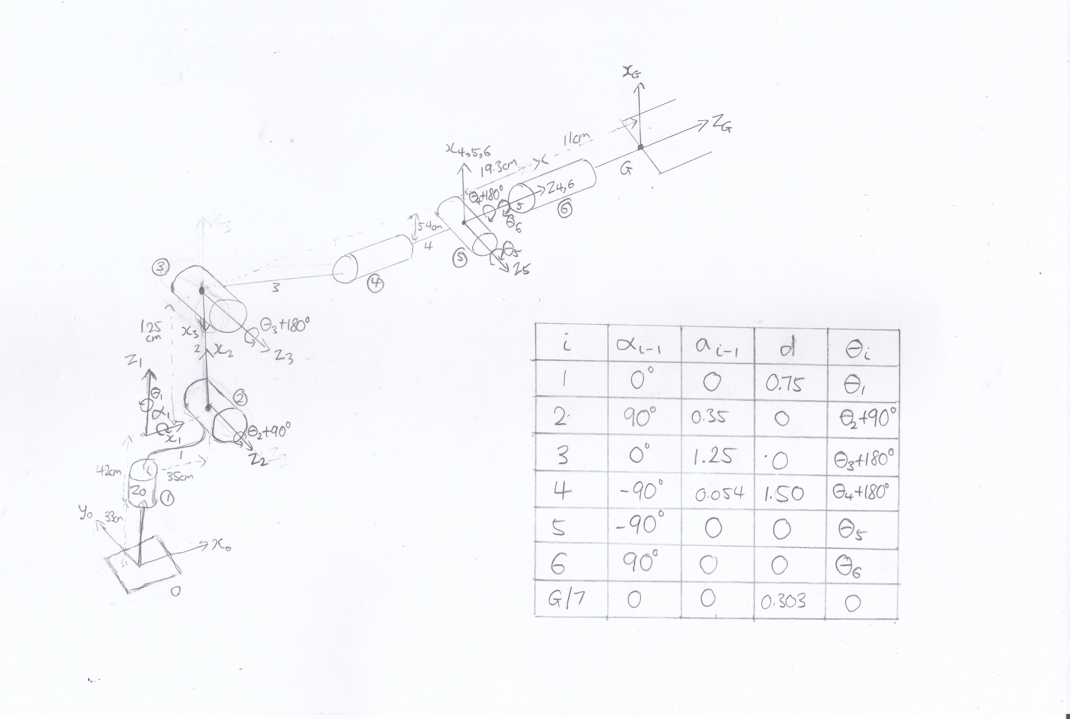
1. Run the forward_kinematics demo and evaluate the kr210.urdf.xacro file to perform kinematic analysis of Kuka KR210 robot and derive its DH parameters.
2. Using the DH parameter table you derived earlier, create individual transformation matrices about each joint. In addition, also generate a generalized homogeneous transform between base_link and gripper_link using only end-effector(gripper) pose.
All the matrices in this section were created using FK_matrices.py.
Individual Transformation Matrices about each joint:
T0_1 : [[cos(theta1), -sin(theta1), 0, 0],
[sin(theta1), cos(theta1), 0, 0], [0, 0, 1, 0.750000000000000], [0, 0, 0, 1]]
T1_2 : [[-sin(theta2), -cos(theta2), 0, 0.350000000000000], [0, 0, -1, 0], [cos(theta2), -sin(theta2), 0, 0], [0, 0, 0, 1]]
T2_3 : [[-cos(theta3), sin(theta3), 0, 1.25000000000000], [-sin(theta3), -cos(theta3), 0, 0], [0, 0, 1, 0], [0, 0, 0, 1]]
T3_4 : [[-cos(theta4), sin(theta4), 0, 0.0540000000000000], [0, 0, 1, 1.50000000000000], [sin(theta4), cos(theta4), 0, 0], [0, 0, 0, 1]]
T4_5 : [[cos(theta5), -sin(theta5), 0, 0], [0, 0, 1, 0], [-sin(theta5), -cos(theta5), 0, 0], [0, 0, 0, 1]]
T5_6 : [[cos(theta6), -sin(theta6), 0, 0], [0, 0, -1, 0], [sin(theta6), cos(theta6), 0, 0], [0, 0, 0, 1]]
T6_EE : [[1, 0, 0, 0], [0, 1, 0, 0], [0, 0, 1, 0.303000000000000], [0, 0, 0, 1]]
The individual transformation matrices are simply evaluated by feeding the DH parameters into the general transformation matrix shown in the lesson Denavit-Hartenberg Parameters.
Assuming that the End-Effector has a position of [px, py ,pz] and has an orientation of euler angles roll, pitch, yaw.
Generalised Homogenous Transform T0_EE:
[[sin(pitch)*cos(roll)*cos(yaw) + sin(roll)*sin(yaw), -sin(pitch)*sin(roll)*cos(yaw) + sin(yaw)*cos(roll), cos(pitch)*cos(yaw), px]
[sin(pitch)*sin(yaw)*cos(roll) - sin(roll)*cos(yaw), -sin(pitch)*sin(roll)*sin(yaw) - cos(roll)*cos(yaw), sin(yaw)*cos(pitch), py]
[cos(pitch)*cos(roll), -sin(roll)*cos(pitch), -sin(pitch), pz]
[0, 0, 0, 1]]
The rotation matrix R0_EE = T0_EE[0:3, 0:3] component is obtained using:
rot_z(yaw) * rot_y(pitch) * rot_x(roll) * rot_y(pi/2) * rot_z(pi)
where rot_y(pi/2) * rot_z(pi) is the angle correction required to align the orientation of the world frame to the resulting gripper frame.
3. Decouple Inverse Kinematics problem into Inverse Position Kinematics and inverse Orientation Kinematics; doing so derive the equations to calculate all individual joint angles.
The wrist center is used for the calculations for the first 3 joints.
Assuming that the wrist center has a position of [wc_x, wc_y, wc_z].
Position
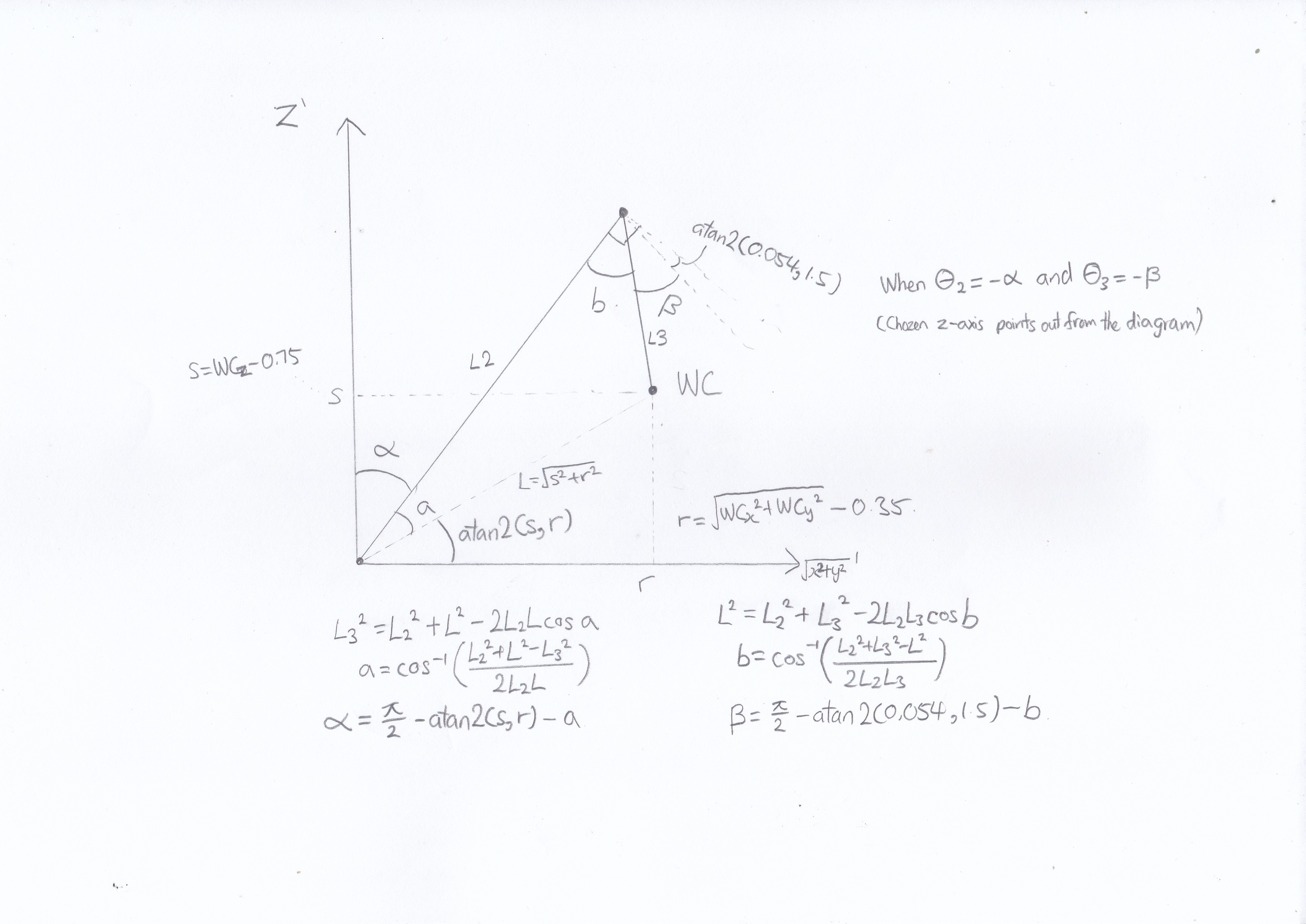
Deriving Theta1 is pretty straightforward since only joint 1 is able to control the z-axis angle.
Theta1 = atan2(wc_y, wc_x)
Deriving Theta2 and Theta3 requires a little more work.

The assumption made here is that L != 0 i.e. the wrist center is not at the origin, which is reasonable since otherwise there would be collisions.
While the diagram only clearly illustrates the situation when 0 <= alpha, beta <= pi/2, it also applies when Theta3 is positive beta and/or Theta2 is positive alpha (-pi/2 <= alpha, beta <= pi/2).
It is also very likely that the magnitude of Theta2 will never need to be more than pi/2 in the context of this problem due to the height of joint 2. Similarly, for Theta3 in the context of this project.
Orientation
Using Forward Kinematics and the angles derived in the position section, we can derive the transformation matrix T0_3, and particularly, we can now obtain the rotation matrix R0_3 from it. Since we derived the generalised Homogenous Transform T0_EE earlier, we can substitute the End-Effector orientation information and obtain a numerically evaluated transformation matrix.
R0_3 * R3_EE = R0_EE
Since inv(R0_3) is the same as transpose(R0_3) (orthonormal),
transpose(R0_3) * R0_3 * R3_EE = transpose(R0_3) * R0_EE
R3_EE = transpose(R0_3) * R0_EE
We are also able to obtain the generalised R3_EE from the forward kinematics matrices:
[[sin(q4)*sin(q6) - cos(q4)*cos(q5)*cos(q6),  sin(q4)*cos(q6) + sin(q6)*cos(q4)*cos(q5), -sin(q5)*cos(q4)],
[                         -sin(q5)*cos(q6),                            sin(q5)*sin(q6),          cos(q5)],
[sin(q4)*cos(q5)*cos(q6) + sin(q6)*cos(q4), -sin(q4)*sin(q6)*cos(q5) + cos(q4)*cos(q6),  sin(q4)*sin(q5)]]
Theta4 = q4 = atan2(r33, -r13)
Theta5 = q5 = atan2(sqrt(r132 + r332), r2,3)
Theta6 = q6 = atan2(r22, -r21)
Of course, since the z-axis chosen is opposite of that used by the software, Thus, Theta2, Theta3 and Theta5 have to be negated before being sent back as response.
1. Fill in the IK_server.py file with properly commented python code for calculating Inverse Kinematics based on previously performed Kinematic Analysis. Your code must guide the robot to successfully complete 8/10 pick and place cycles. Briefly discuss the code you implemented and your results.
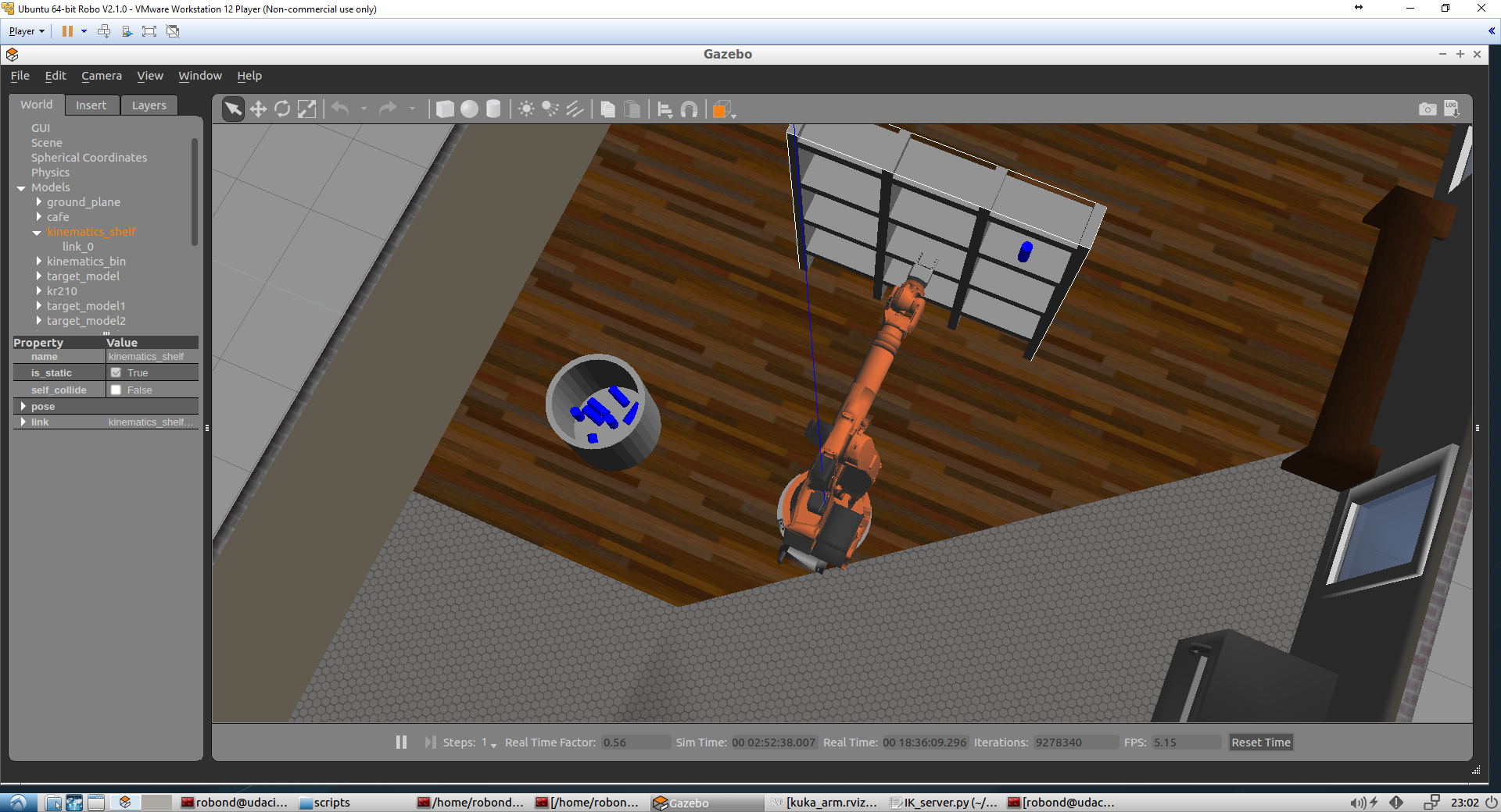
So far it has been performing pretty successfully after adding a delay to the gripping. Since I stuck to the parameters/algorithm described in the lessons, I ended up using a z-axis in the opposite direction of the software. The negation got me really confused at times (and wasted alot of time...), but finally managed to sort it out.
Here is a picture that I sent to some of my friends. :p
Also, since the error computation of the End-Effector position is rather straightforward (unless it meant collecting data and doing some statistical analysis...), I implemented it and my error values seem to be in the magnitude of 10-16m!

