Traffic Sign Recognition

Build a Traffic Sign Recognition Project

The goals / steps of this project are the following:

Load the data set (see below for links to the project data set)
Explore, summarize and visualize the data set
Design, train and test a model architecture
Use the model to make predictions on new images
Analyze the softmax probabilities of the new images
Summarize the results with a written report

Data Set Summary & Exploration

1. Provide a basic summary of the data set. In the code, the analysis should be done using python, numpy and/or pandas methods rather than hardcoding results manually.

I used the pandas library to calculate summary statistics of the traffic signs data set:

The size of training set is 34799
The size of the validation set is 4410
The size of test set is 12630
The shape of a traffic sign image is (34799, 32, 32, 3)
The number of unique classes/labels in the data set is 43

2. Visualization of the dataset.

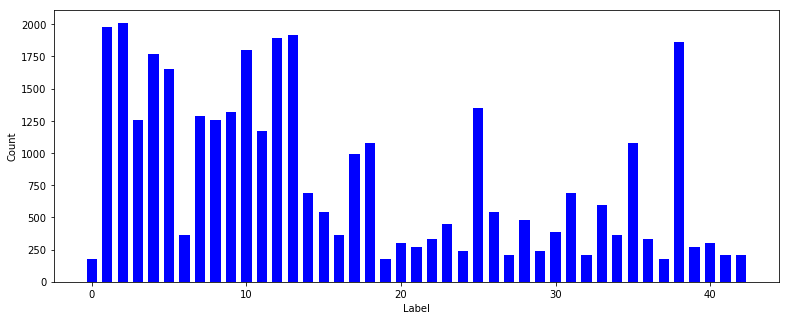
Here is an exploratory visualization of the data set. It is a bar chart showing the number of images over the labels.

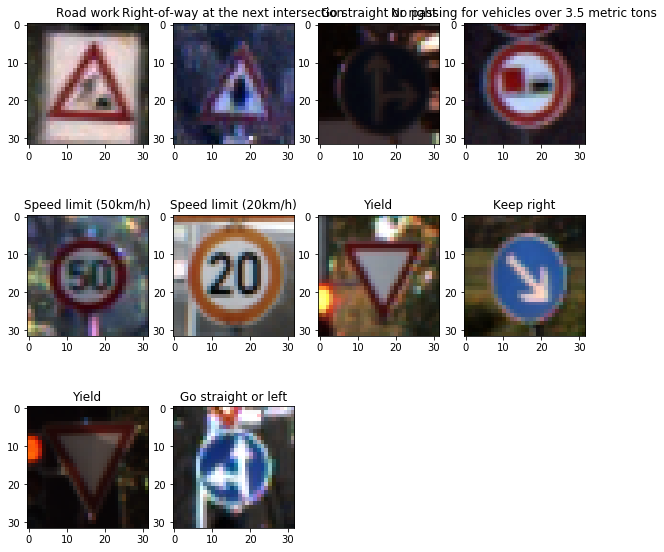
Design and Test a Model Architecture

1. Preprocess part

As a last step, I normalized the image data using openCV min max normalizer to get a better contrast.

Here is a sample of normalized images:

2. Model architecture

My final model consisted of the following layers:

Layer	Description
Input	32x32x3 RGB image
Convolution 5x5	1x1 stride, valid padding, outputs 28x28x6
RELU
Max pooling	2x2 stride, outputs 14x14x6
Normalization
Convolution 5x5	1x1 stride, valid padding, outputs 10x10x16
RELU
Normalization
Max pooling	2x2 stride, outputs 5x5x16
Flatten	output 400
Fully connected	output 120
Fully connected	output 84
Dropout	probability : 0.5
Softmax	outpur 43

3. How I trained my model.

The model is based on Lenet with some inspiration from Cifar-10 such as include normalization layers. The learning rate is 0.0005 to avoid being stuck in local optimum. The number of epochs is 15 to compensate a small learning rate. I used the Adam optimizer with a batch size of 128 to avoid memory issues.

4. My approach

My final model results were:

training set accuracy of 0.994
validation set accuracy of 0.964
test set accuracy of 0.947

I used an iterative approach, I started my project with a Lenet architecture, then add features from Cifar-10 (normalization layers at strategic points, I tried after the first pooling layer and after the second conv layer) and then add a last dropout layer. The first achitecture (Lenet) had an accuracy of 0.85, the next one had 0.93 (with normalizers) and finaly 0.96 with dropout due to possible overfitting. I also tried a valid padding to get smaller outputs to accelerate the trainning without too much loss. I think the first convolution layer with valid padding is a good thing to the neural network to focus on the center of the image. Combine convolution layers with pooling layers is also very effective.

Test a Model on New Images

Here are 16 German traffic signs that I found on the web, from http://benchmark.ini.rub.de/?section=gtsrb&subsection=dataset:

I think the image with 30km/h speed limit should be difficult to classify because it's very noisy.

2. model's predictions on these new traffic signs

Here are the results of the prediction:

Image	Prediction
Yield	Yield
Yield	Yield
Bumpy road	Bumpy road
Slippery road	Slippery road
Speed limit (100km/h)	Speed limit (80km/h)
Roundabout mandatory	Roundabout mandatory
General caution	General caution
Right-of-way at the next intersection	Right-of-way at the next intersection
Speed limit (70km/h)	Speed limit (70km/h)
Vehicles over 3.5 metric tons prohibited	End of no passing
No entry	No entry
Priority road	Priority road
Ahead only	Ahead only
Speed limit (30km/h)	Speed limit (30km/h)
Traffic signals	Traffic signals

The model was able to correctly guess 14 of the 16 traffic signs, which gives an accuracy of 87.5%. This is less than previous accuracies from test, validation and train sets.

3. How certain the model is when predicting on each of the 16 new images by looking at the softmax probabilities for each prediction.

The code for making predictions on my final model is located in the 17th cell of the Jupyter notebook.

Finally, the sign 30km/h speed limit was not a problem compared to 100km/h speed limit sign. The top five soft max probabilities were:

INFO:tensorflow:Restoring parameters from ./lenet Yield was predicted :

Yield at 0.9997619986534119%
Speed limit (50km/h) at 0.0001685354218352586%
Road work at 3.1417046557180583e-05%

Yield was predicted :

Yield at 0.9999943971633911%
Speed limit (30km/h) at 3.6590374747902388e-06%
Keep right at 8.095304337984999e-07%

Stop was predicted :

Stop at 0.9997864365577698%
Speed limit (80km/h) at 0.00017442155512981117%
Speed limit (30km/h) at 1.4265858226281125e-05%

Bumpy road was predicted :

Bumpy road at 0.9658303260803223%
Road narrows on the right at 0.01878529228270054%
Dangerous curve to the right at 0.007164016831666231%

Slippery road was predicted :

Slippery road at 0.9042190313339233%
Dangerous curve to the left at 0.06443075835704803%
Dangerous curve to the right at 0.026664407923817635%

Speed limit (100km/h) was predicted :

Speed limit (80km/h) at 0.6539806723594666%
Speed limit (100km/h) at 0.33548855781555176%
Vehicles over 3.5 metric tons prohibited at 0.00474350294098258%

Roundabout mandatory was predicted :

Roundabout mandatory at 0.9944174289703369%
Go straight or left at 0.004873400554060936%
Keep right at 0.0005993542145006359%

General caution was predicted :

General caution at 0.9966030120849609%
Traffic signals at 0.0032088051084429026%
Pedestrians at 0.00017882279644254595%

Right-of-way at the next intersection was predicted :

Right-of-way at the next intersection at 0.9991012811660767%
Beware of ice/snow at 0.0008936773519963026%
Children crossing at 3.6047531466465443e-06%

Speed limit (70km/h) was predicted :

Speed limit (70km/h) at 0.9986227750778198%
Speed limit (30km/h) at 0.001275851740501821%
No vehicles at 5.338023402146064e-05%

Vehicles over 3.5 metric tons prohibited was predicted :

End of no passing at 0.9328629970550537%
End of all speed and passing limits at 0.031764477491378784%
End of no passing by vehicles over 3.5 metric tons at 0.008638669736683369%

No entry was predicted :

No entry at 0.9995668530464172%
Stop at 0.00042210103129036725%
No vehicles at 6.8793524405919015e-06%

Priority road was predicted :

Priority road at 0.9968223571777344%
Yield at 0.0025436219293624163%
End of all speed and passing limits at 0.00043486038339324296%

Ahead only was predicted :

Ahead only at 0.9999457597732544%
Turn right ahead at 1.8656082829693332e-05%
Turn left ahead at 1.6260117263300344e-05%

Speed limit (30km/h) was predicted :

Speed limit (30km/h) at 0.9457525014877319%
Speed limit (50km/h) at 0.05390146002173424%
Speed limit (70km/h) at 0.0001552138419356197%

Traffic signals was predicted :

Traffic signals at 0.9706506133079529%
General caution at 0.017575105652213097%
Road narrows on the right at 0.009173298254609108%

The sign "Vehicles over 3.5 metric tons prohibited" wasn't predicted correctly, I think it's due to the short number of this sign labelised.

maggiemhanna/Traffic_Sign_Classifier