Extended documentation can be found on the website: https://majkamichal.github.io/naivebayes/
The naivebayes package presents an efficient implementation of the
widely-used Naïve Bayes classifier. It upholds three core principles:
efficiency, user-friendliness, and reliance solely on Base R. By
adhering to the latter principle, the package ensures stability and
reliability without introducing external dependencies1. This design
choice maintains efficiency by leveraging the optimized routines
inherent in Base R, many of which are programmed in high-performance
languages like C/C++ or FORTRAN. By following these principles, the
naivebayes package provides a reliable and efficient tool for Naïve
Bayes classification tasks, ensuring that users can perform their
analyses effectively and with ease.
The naive_bayes() function is designed to determine the class of each
feature in a dataset, and depending on user specifications, it can
assume various distributions for each feature. It currently supports the
following class conditional distributions:
- categorical distribution for discrete features (with Bernoulli distribution as a special case for binary outcomes)
- Poisson distribution for non-negative integer features
- Gaussian distribution for continuous features
- non-parametrically estimated densities via Kernel Density Estimation for continuous features
In addition to that specialized functions are available which implement:
- Bernoulli Naive Bayes via
bernoulli_naive_bayes() - Multinomial Naive Bayes via
multinomial_naive_bayes() - Poisson Naive Bayes via
poisson_naive_bayes() - Gaussian Naive Bayes via
gaussian_naive_bayes() - Non-Parametric Naive Bayes via
nonparametric_naive_bayes()
These specialized functions are carefully optimized for efficiency,
utilizing linear algebra operations to excel when handling dense
matrices. Additionally, they can also exploit sparsity of matrices for
enhanced performance and work in presence of missing data. The package
also includes various helper functions to improve user experience.
Moreover, users can access the general naive_bayes() function through
the excellent Caret package, providing additional versatility.
The naivebayes package can be installed from the CRAN repository by
simply executing in the console the following line:
install.packages("naivebayes")

# Or the the development version from GitHub:
devtools::install_github("majkamichal/naivebayes")The naivebayes package provides a user friendly implementation of the
Naïve Bayes algorithm via formula interlace and classical combination of
the matrix/data.frame containing the features and a vector with the
class labels. All functions can recognize missing values, give an
informative warning and more importantly - they know how to handle them.
In following the basic usage of the main function naive_bayes() is
demonstrated. Examples with the specialized Naive Bayes classifiers can
be found in the extended documentation:
https://majkamichal.github.io/naivebayes/ in this
article.
library(naivebayes)
#> naivebayes 1.0.0 loaded
#> For more information please visit:
#> https://majkamichal.github.io/naivebayes/

# Simulate example data
n <- 100
set.seed(1)
data <- data.frame(class = sample(c("classA", "classB"), n, TRUE),
                   bern = sample(LETTERS[1:2], n, TRUE),
                   cat  = sample(letters[1:3], n, TRUE),
                   logical = sample(c(TRUE,FALSE), n, TRUE),
                   norm = rnorm(n),
                   count = rpois(n, lambda = c(5,15)))
train <- data[1:95, ]
test <- data[96:100, -1]nb <- naive_bayes(class ~ ., train)
summary(nb)
#>
#> ================================= Naive Bayes ==================================
#>
#> - Call: naive_bayes.formula(formula = class ~ ., data = train)
#> - Laplace: 0
#> - Classes: 2
#> - Samples: 95
#> - Features: 5
#> - Conditional distributions:
#> - Bernoulli: 2
#> - Categorical: 1
#> - Gaussian: 2
#> - Prior probabilities:
#> - classA: 0.4842
#> - classB: 0.5158
#>
#> --------------------------------------------------------------------------------
# Classification
predict(nb, test, type = "class")
#> [1] classA classB classA classA classA
#> Levels: classA classB
nb %class% test
#> [1] classA classB classA classA classA
#> Levels: classA classB
# Posterior probabilities
predict(nb, test, type = "prob")
#> classA classB
#> [1,] 0.7174638 0.2825362
#> [2,] 0.2599418 0.7400582
#> [3,] 0.6341795 0.3658205
#> [4,] 0.5365311 0.4634689
#> [5,] 0.7186026 0.2813974
nb %prob% test
#> classA classB
#> [1,] 0.7174638 0.2825362
#> [2,] 0.2599418 0.7400582
#> [3,] 0.6341795 0.3658205
#> [4,] 0.5365311 0.4634689
#> [5,] 0.7186026 0.2813974
# Helper functions
tables(nb, 1)
#> --------------------------------------------------------------------------------
#> :: bern (Bernoulli)
#> --------------------------------------------------------------------------------
#>
#> bern classA classB
#> A 0.5000000 0.5510204
#> B 0.5000000 0.4489796
#>
#> --------------------------------------------------------------------------------
get_cond_dist(nb)
#> bern cat logical norm count
#> "Bernoulli" "Categorical" "Bernoulli" "Gaussian" "Gaussian"
# Note: all "numeric" (integer, double) variables are modelled
# with Gaussian distribution by default.X <- train[-1]
class <- train$class
nb2 <- naive_bayes(x = X, y = class)
nb2 %prob% test
#> classA classB
#> [1,] 0.7174638 0.2825362
#> [2,] 0.2599418 0.7400582
#> [3,] 0.6341795 0.3658205
#> [4,] 0.5365311 0.4634689
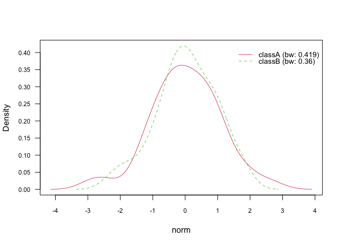
#> [5,] 0.7186026 0.2813974Kernel density estimation can be used to estimate class conditional
densities of continuous features. It has to be explicitly requested via
the parameter usekernel=TRUE otherwise Gaussian distribution will be
assumed. The estimation is performed with the built in R function
density(). By default, Gaussian smoothing kernel and Silverman’s rule
of thumb as bandwidth selector are used:
nb_kde <- naive_bayes(class ~ ., train, usekernel = TRUE)
summary(nb_kde)
#>
#> ================================= Naive Bayes ==================================
#>
#> - Call: naive_bayes.formula(formula = class ~ ., data = train, usekernel = TRUE)
#> - Laplace: 0
#> - Classes: 2
#> - Samples: 95
#> - Features: 5
#> - Conditional distributions:
#>     - Bernoulli: 2
#>     - Categorical: 1
#>     - KDE: 2
#> - Prior probabilities:
#>     - classA: 0.4842
#>     - classB: 0.5158
#>
#> --------------------------------------------------------------------------------
get_cond_dist(nb_kde)
#>          bern           cat       logical          norm         count
#>   "Bernoulli" "Categorical"   "Bernoulli"         "KDE"         "KDE"
nb_kde %prob% test
#>         classA    classB
#> [1,] 0.6498111 0.3501889
#> [2,] 0.2279460 0.7720540
#> [3,] 0.5915046 0.4084954
#> [4,] 0.5876798 0.4123202
#> [5,] 0.7017584 0.2982416

# Class conditional densities
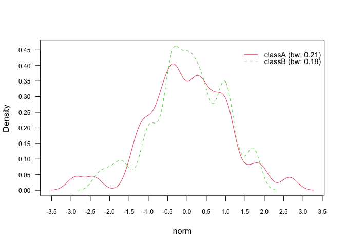
plot(nb_kde, "norm", arg.num = list(legend.cex = 0.9), prob = "conditional")
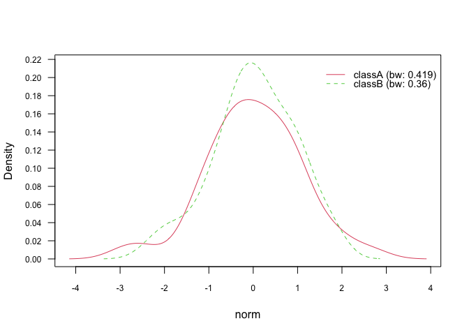
# Marginal densities
plot(nb_kde, "norm", arg.num = list(legend.cex = 0.9), prob = "marginal")In general, there are 7 different smoothing kernels available:
gaussianepanechnikovrectangulartriangularbiweightcosineoptcosine
and they can be specified in naive_bayes() via parameter additional
parameter kernel. Gaussian kernel is the default smoothing kernel.
Please see density() and bw.nrd() for further details.
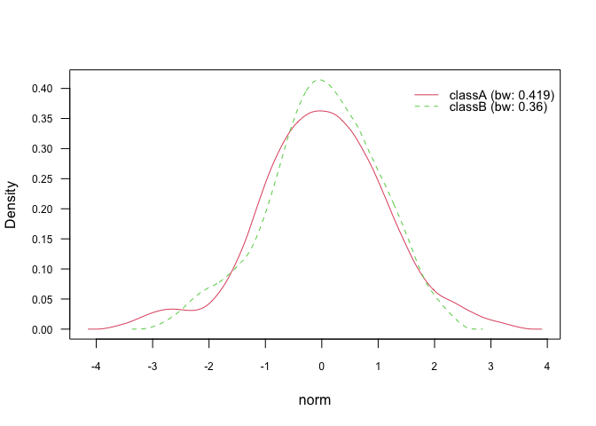
# Change Gaussian kernel to biweight kernel
nb_kde_biweight <- naive_bayes(class ~ ., train, usekernel = TRUE,
                               kernel = "biweight")
nb_kde_biweight %prob% test
#>         classA    classB
#> [1,] 0.6564159 0.3435841
#> [2,] 0.2350606 0.7649394
#> [3,] 0.5917223 0.4082777
#> [4,] 0.5680244 0.4319756
#> [5,] 0.6981813 0.3018187
plot(nb_kde_biweight, "norm", arg.num = list(legend.cex = 0.9), prob = "conditional")The density() function offers 5 different bandwidth selectors, which
can be specified via bw parameter:
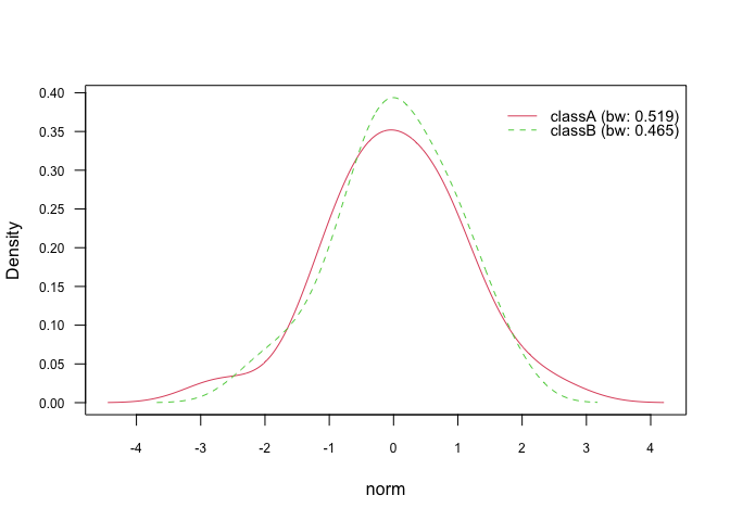
nrd0(Silverman’s rule-of-thumb)nrd(variation of the rule-of-thumb)ucv(unbiased cross-validation)bcv(biased cross-validation)SJ(Sheather & Jones method)
nb_kde_SJ <- naive_bayes(class ~ ., train, usekernel = TRUE,
                               bw = "SJ")
nb_kde_SJ %prob% test
#>         classA    classB
#> [1,] 0.6127232 0.3872768
#> [2,] 0.1827263 0.8172737
#> [3,] 0.5784831 0.4215169
#> [4,] 0.7031048 0.2968952
#> [5,] 0.6699132 0.3300868
plot(nb_kde_SJ, "norm", arg.num = list(legend.cex = 0.9), prob = "conditional")The parameter adjust allows to rescale the estimated bandwidth and
thus introduces more flexibility to the estimation process. For values
below 1 (no rescaling; default setting) the density becomes “wigglier”
and for values above 1 the density tends to be “smoother”:
nb_kde_adjust <- naive_bayes(class ~ ., train, usekernel = TRUE,
                         adjust = 0.5)
nb_kde_adjust %prob% test
#>         classA    classB
#> [1,] 0.5790672 0.4209328
#> [2,] 0.2075614 0.7924386
#> [3,] 0.5742479 0.4257521
#> [4,] 0.6940782 0.3059218
#> [5,] 0.7787019 0.2212981
plot(nb_kde_adjust, "norm", arg.num = list(legend.cex = 0.9), prob = "conditional")Class conditional distributions of non-negative integer predictors can
be modelled with Poisson distribution. This can be achieved by setting
usepoisson=TRUE in the naive_bayes() function and by making sure
that the variables representing counts in the dataset are of class
integer.
is.integer(train$count)
#> [1] TRUE
nb_pois <- naive_bayes(class ~ ., train, usepoisson = TRUE)
summary(nb_pois)
#>
#> ================================= Naive Bayes ==================================
#>
#> - Call: naive_bayes.formula(formula = class ~ ., data = train, usepoisson = TRUE)
#> - Laplace: 0
#> - Classes: 2
#> - Samples: 95
#> - Features: 5
#> - Conditional distributions:
#>     - Bernoulli: 2
#>     - Categorical: 1
#>     - Poisson: 1
#>     - Gaussian: 1
#> - Prior probabilities:
#>     - classA: 0.4842
#>     - classB: 0.5158
#>
#> --------------------------------------------------------------------------------
get_cond_dist(nb_pois)
#>          bern           cat       logical          norm         count
#>   "Bernoulli" "Categorical"   "Bernoulli"    "Gaussian"     "Poisson"

nb_pois %prob% test
#>         classA    classB
#> [1,] 0.6708181 0.3291819
#> [2,] 0.2792804 0.7207196
#> [3,] 0.6214784 0.3785216
#> [4,] 0.5806921 0.4193079
#> [5,] 0.7074807 0.2925193

# Class conditional distributions
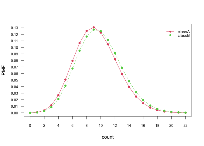
plot(nb_pois, "count", prob = "conditional")
# Marginal distributions
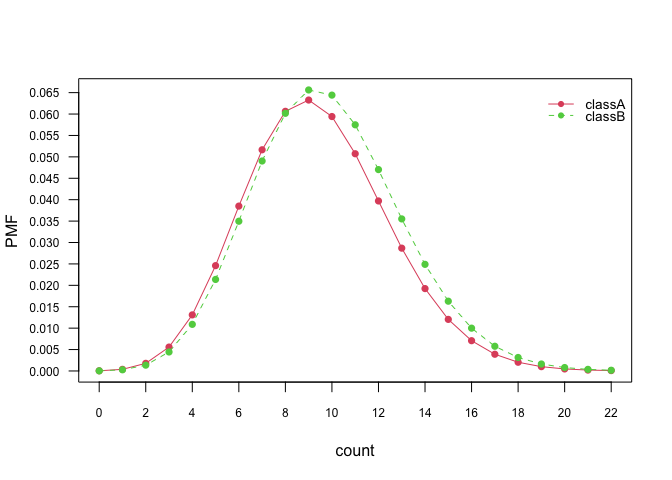
plot(nb_pois, "count", prob = "marginal")Footnotes
-
Specialized Naïve Bayes functions within the package may optionally utilize sparse matrices if the Matrix package is installed. However, the Matrix package is not a dependency, and users are not required to install or use it. ↩


