SLAPStack is a block-stacking warehouse simulation for the Autonomous Block Stacking Warehouse Problem (ABSWP) [1] implementing the OpenAI gym interface. The code can be used to test out Storage Location Allocation Problem (SLAP) and Unit Load Selection Problem (ULSP) algorithms individually or in conjunction.
The simulation project includes the WEPAStacks data which includes the layout
and 3 months of order information of a large-scale real-world clock stacking
warehouse from WEPA Hygieneprodukte GmbH.
Additionally, an anonymized use case dataset, CrossStacks associated with a
medium-sized cross-docking terminal is made available. CrossStacks
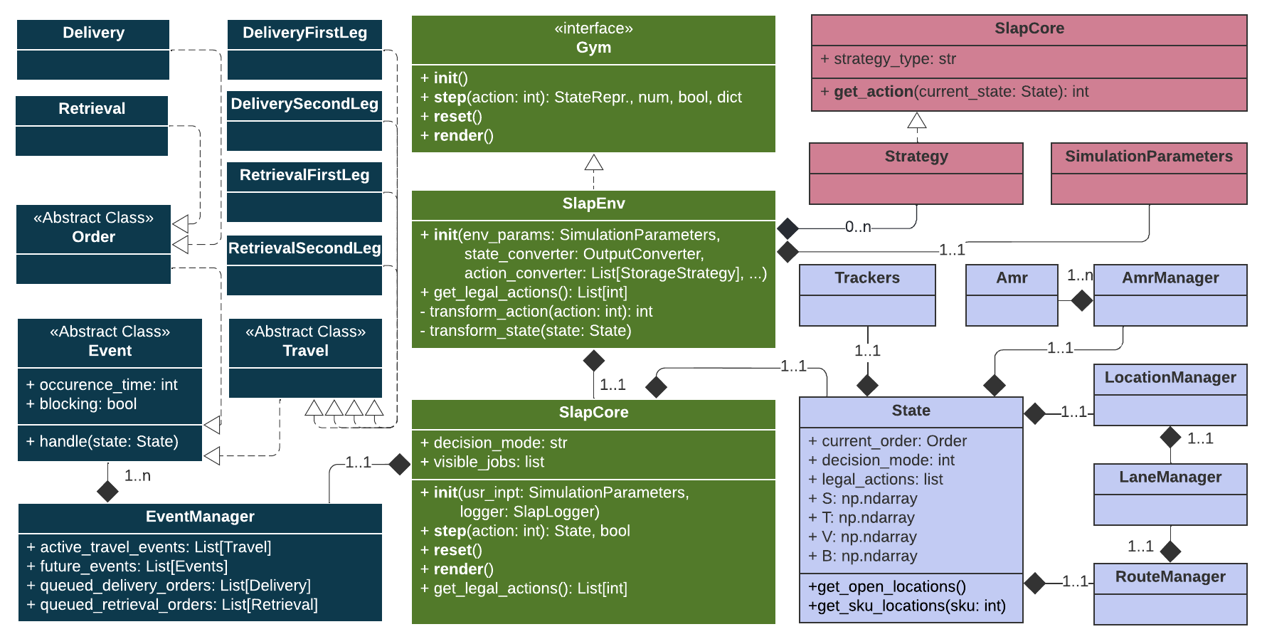
The project architecture follows the one introduced in [2],
as can be seen in the partial class diagram below. The simulation entry point,
which implements the gym interface is located in the SlapEnv class located in
the interface.py module. SlapEnv, whose primary function is action- and
state-space configuration and transformation, is a wrapper around the SlapCore
which contains the simulation logic.
SlapCore is responsible for advancing the simulation when calling step. It
uses an EventManager object to maintain the Event queues. The central
SLAPStack communication structure is given by the State object contained by
the SlapCore.
The State contains several manager objects dedicated to distinct tasks.
The RouteManager, for instance, is used to compute routes on the storage
matrix S grid during Transport event initialization. The 3D state matrices
S (pallet SKUs information), V (vehicle positions),
B (pallet batch information), and T (pallet arrival information) are shared
between State and manager objects as needed (e.g. V is shared between
AmrManager and State).
The interface_templates.py module defines and documents the simulation
parameter as well as the SlapEnv configuration objects, i.e. Strategy for
allowing indirect actions and OutputConverter for transforming both the state
representation and the reward returned by SlapEnv.step().
At the core of the simulation lies the future_events queue. future_events is
a time-sorted heap of self-handling events. During a simulation step, events are
popped from this heap and their handle function is called leading to a state
update. If a triggered event requires an external ULSP or SLAP decision, the
execution halts, and the state is returned.
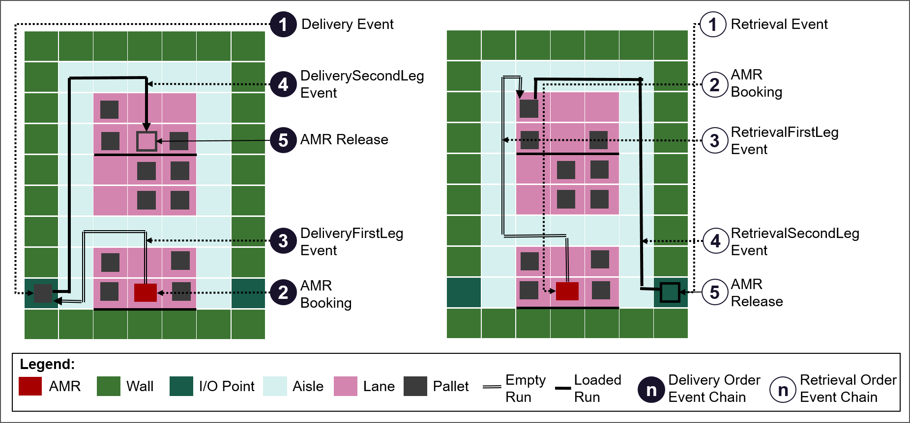
Events are either orders or transport events. Orders (Delivery or Retrieval)
get added to the queue during initialization. Transport events
(Delivery/RetrievalFirst/SecondLeg) are created on-demand. Of the 6 events
present in the simulation, 2 are blocking, namely Retrieval and
DeliverySecondLeg. The relationship between them is depicted event chain
summary below.
The design lain down in [2] and implemented by SLAPStack leads
to an efficient runtime in terms of event management and state updates.
All state updates are run in constant or amortized constant time.
Since, future_events is a binary heap, pushing Order events to it during
initialization and Transport events to it during step takes logarithmic
time with respect to the total number of orders. This yields an asymptotic
runtime of O(n log(n)), where n is the number of orders.
However, a particularity of SLAPStack is the fine-grained routing mechanism
implemented. Whenever a Transport event is created, the exact closest grid
cell route between the AMRs current position and its destination is computed.
Dijkstra takes O(m log(m + l)) where m is the number of nodes and l is the
number of edges in the routing graph. In our case, that would amount to
O(m log m) with m being the number of grid cells in the BSWP (each grid cell is
a routing graph node and each cell has four bidirectional edges,
i.e. O(m log(m + l) = O(m log(m + 4m)) = O(m log(m)).
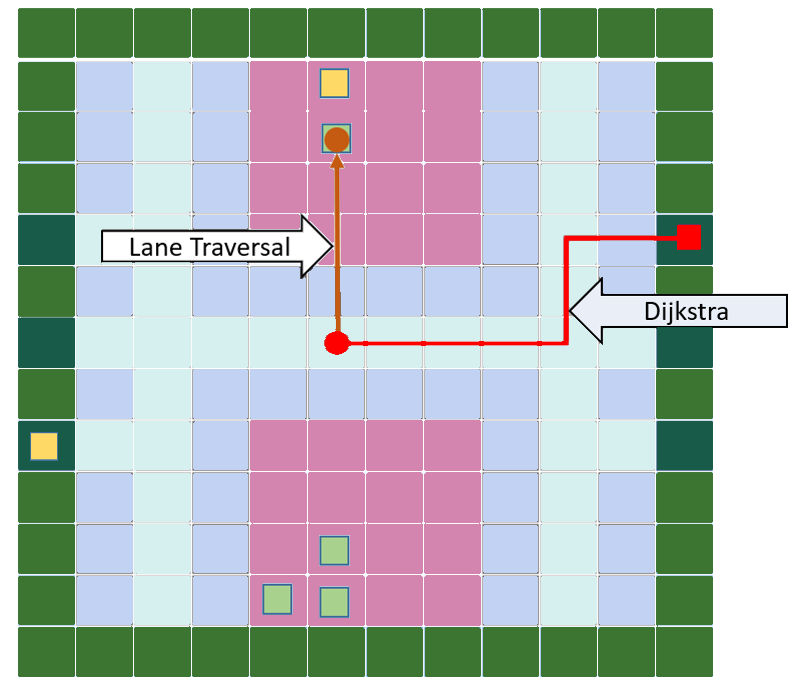
To deal with this routing bottleneck, SLAPStack's RouteManager precomputes
all routes over aisle tiles (the light blue tiles in the figure below) using
the Floyed Warshall algorithm implemented in scipy. The exact route
computation is then completed by adding lane traversal segments which runs in
constant time (see figure).
Simulating a total of 400000 orders on CPU take around 1 hour.
The latest version of this simulation contains extensions necessary to accommodate cross-docking use-cases and dual command cycle heuristics. These extensions are:
- dock to dock transports
- order queueing on AMRs
Additionally, AMRs are capable or transporting more than one load at a time (multiple forks).
This dataset is based on a real-world block stacking warehouse from WEPA.
WEPA is one of the largest hygienic paper manufacturers in Europe with production plants and warehouses in currently six European countries (www.wepa.eu).
The dataset consists of three components:
- the warehouse layout
- the initial fill level
- the order stream
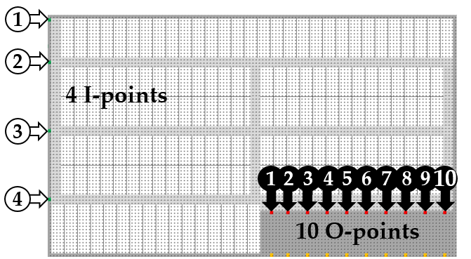
The grid-based warehouse layout shown in the figure below is used to store finished goods on standardized EUR-pallets that can be stacked up to 3 levels. The capacity of the warehouse is up to 19512 storage locations (6504 on the ground with stacking). The light-gray area shows the bidirectional pathways (aisles). Dependent on the type of vehicle they are double/three-lanes wide. The storage bays/lanes are the white areas with separating lines. The dark-gray surrounding wall and truck loading zone define the boundaries of the storage system. Interfaces to the outside world are 4 Inputs (I-points) that represent the production lines and 10 Outputs (O-points) for shipping. At I-points the delivered pallets are picked up and transported to a storage location. Upon the arrival of a retrieval order, pallets are provided at the O-points. O-points are the staging areas in front of the dock doors. The truck loading process is not part of the use-case since it is executed by the truck drivers.
The warehouse layout is provided as csv-file with numbers from -5 to 0. A -5 represents a travel path, -4 an O-point, -3 an I-point, -2 an aisle, -1 the warehouse boundaries and 0 the available storage locations.
The initial fill level is a dictionary of Stock Keeping Unit (SKUs) with the respective amount currently on stock at time zero.
The order stream represents the daily in- and outbound flow with the exact arrival times of each delivery or retrieval order for a time period of 89 days (amounting to 4e5 orderes). Each order corresponds to a single pallet. While the inbound flow is based on a production frequency of 60 to 120 seconds, the outbound flow is mainly in full truck loads (FTL) with 33 pallets.
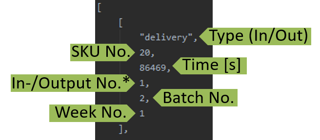
The orders are provided as a nested list. Each order comes with six parameters namely the type (delivery or retrieval), the SKU (number from 1 to 136), the order arrival time (absolute time in seconds counting from zero), the dock door (number from 1 to 4 from top to bottom for delivery and 1 to 10 from left to right for retrieval), the batch number (number of production batches from 1 to 1498 for delivery and of truckload batches from 1 to 7496 for retrieval) and the week number (from 1 to 14).
CROSSStacks, that was constructed based on two weeks of orders of a
medium-sized, manually operated cross-docking terminal for food industry goods
run by a large freight company. The data we provide was gathered with the help
of a process mining company focusing on increasing the transparency of (manual)
industrial processes without revealing any sensitive customer information.
As opposed to WEPAStacks the CrossStacks dataset consists of only two
components, bacause the warehouse is empty at the beginning of a new day.
- the warehouse layout
- the order stream
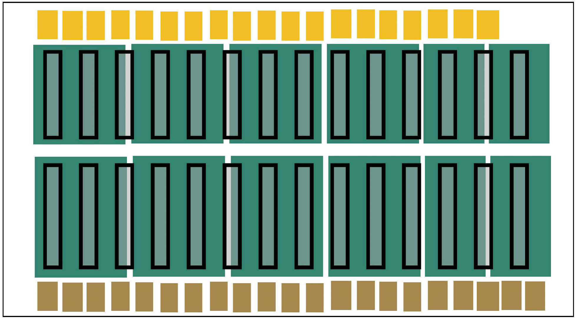
The figure below depicts an overlay of the warehouse layout and storage regions tracked by the process mining company. Yellow boxes represent inbound docks, brown boxes represent outboutnd docks. The storage bays are represented by empty black rectangles. The green-filled rectangles represent the storage regions tracked by the process mining company. Within the current use case stacking is not allowed.
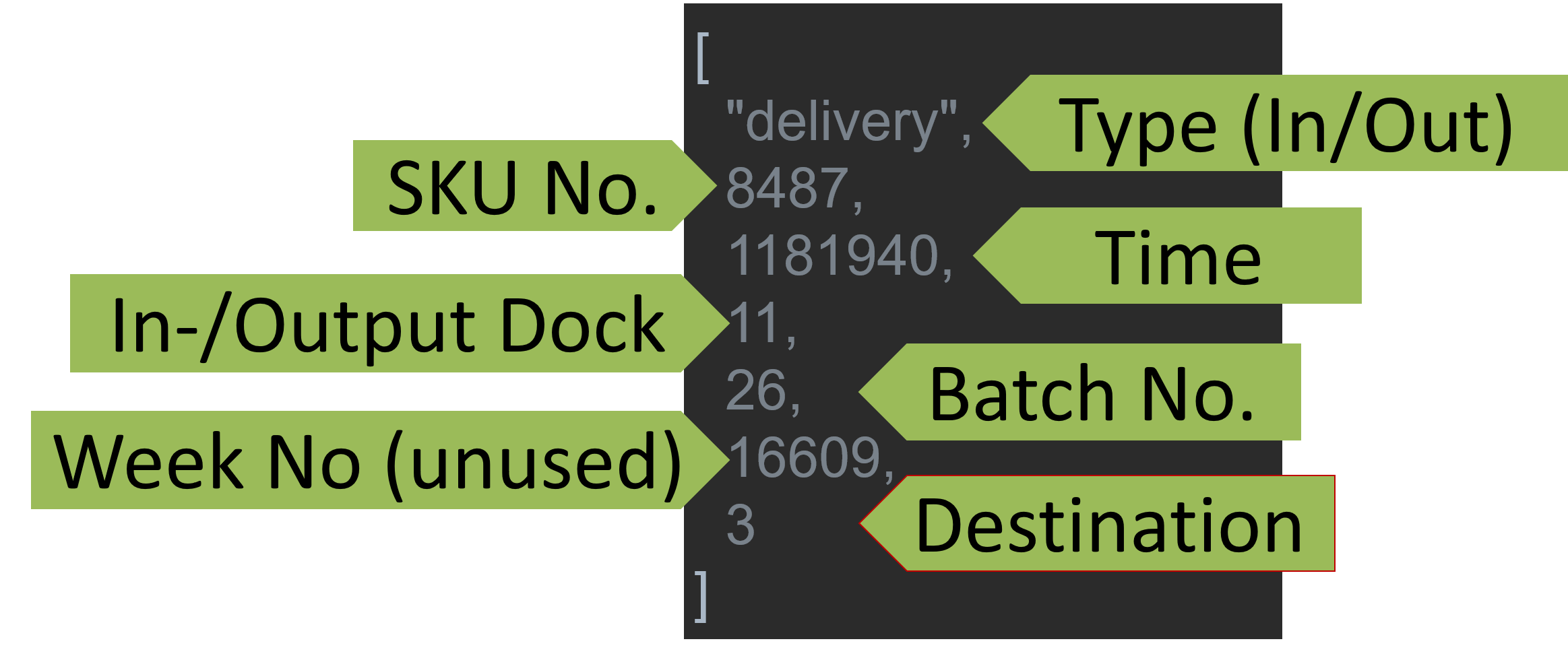
Cross-docking orders contain add a sixth field, namely the destination dock, to the structure previously described (cmp. figure below). This field is only relevant for delivery orders.
The destination field was unavailable to us in an explicit form and needed to be inferred from the data. To that end, we used the motion tracking information together with a FIFO assumption to extract the destination dock of inbound orders: We aligned the orders entering and exiting the green storage regions in the layout figures using tracking timestamps and assigned the outbound docks to the corresponding inbound orders.
This package contains several control heuristics associated with the SLAPStack
block stacking warehouse (BSW) simulation. The code is hosted together with the
simulation on github.
SLAPStack contains two use cases, namely WEPAStacks and Crossstacks.
See the linked repository for more information.
For WEPAStacks, the following storage location allocation problem (SLAP)
strategies were implemented and tested (a comparison of these strategies is
available through [3]):
- Closest open pure lane (COPL) and
- Class-based popularity with the following stock keeping unit (SKU) popularity
measures:
- SKU turnover time (indirectly proportional to popularity)
- The historic number of picks per SKU (directly proportional to popularity)
- The number of future SKU picks over the next planning period, e.g. week (directly proportional to popularity)
- The historic SKU throughput calculated as the sum of picks and deliveries per SKU (directly proportional to popularity)
- The future SKU throughput over the next planning period
For CrossStacks (publication pending), the implemented strategies are:
- Closest to destination (CTD),
- Closest open location (COL),
- Random location (RND), and
- Two dual command cycle inspired heuristics:
- Closest to the next delivery order (CTNR)
- Shortest leg (SL)
Note that the CrossStacks SLAP strategies could be applied to the WEPAStacks
use case and vice-versa, however this application has not yet been tested.
The following unit load selection problem (ULSP) policies are implemented:
- Batch Last In First Out (BLIFO)
We publish this project alongside our experiment script and a control package containing various SLAP heuristics as well as a ULSP heuristic. To set up your environment and recreate our experiment results, the following steps can be taken:
- Cloning the repository:
git clone https://github.com/malerinc/slapstack.git - To install the SLAPStack simulation and its controls run the following commands from the project root directory (this will build the Cython extensions and copy the use case data at the appropriate locations):
pip install 1_environment/slapstack pip install 2_control/slapstack-controls - To run the experiment script, simply execute the
cmpscripts located in the experiments directory directly under the root:python slap_strategy_cmp_crossstacks.py python slap_strategy_cmp_wepastacks.py
Note that both the slapstack and slapstack-controls packages are available
through pypi as well. To install from pypi, simply run
pip install slapstack
pip install slapstack-controls
If you use SLAPStack, WEPAStacks or CrossStacks in your research, you can
cite this repository as follows:
@misc{rinciog2023slapstack
    author = {Rinciog, Alexandru and Pfrommer, Jakob and Morrissey Michael
      and Sohaib Zahid and Vasileva, Anna and Ogorelysheva, Natalia and
      Rathod, Hardik and Meyer Anne},
    title = {SLAPStack},
    year = {2023},
    publisher = {GitHub},
    journal = {GitHub Repository},
    howpublished = {\url{https://github.com/malerinc/slapstack.git}},
}
[1] Pfrommer, J., Meyer, A.: Autonomously organized block stacking warehouses: A review of decision problems and major challenges. Logistics Journal: Proceedings 2020(12) (2020)
[2] Rinciog, A., Meyer, A.: Fabricatio-rl: A reinforcement learning simulation framework for production scheduling. In: 2021 Winter Simulation Conference (WSC). pp. 1–12. IEEE (2021)
[3] Pfrommer, J.; Rinciog, A.; Zahid, S.; Morrissey, M; Meyer A. (2022): SLAPStack: A Simulation Framework and a Large-Scale Benchmark Use Case for Autonomous Block Stacking Warehouses. International Conference on Computational Logistics (ICCL) 2022.

