QuantumSpatialSearch

QuantumSpatialSearch simulates a spatial search algorithm using a continuous time quantum walk (CTQW) on an arbitrary graph, described by its adjacency matrix. It also simulates the effects of dynamic random telegraph noise (RTN) affecting the links of the graph, by Montecarlo-sampling the noise and averaging the quantum trajectory.

This Julia 1.0 package is used to obtain the numerical results of the manuscript M. Cattaneo, M. A. C. Rossi, M. G. A. Paris, S. Maniscalco, Quantum spatial search on graphs with dynamical noise, arXiv:1809.01969.

Installation

You can install the package using the Pkg-REPL, which is entered from the Julia REPL using the key ].

(v1.0) pkg> add https://github.com/matteoacrossi/QuantumSpatialSearch.git

You can then test that everything works as expected

(v1.0) pkg> test QuantumSpatialSearch

Usage

The main function is spatialsearch

        (p, t, pmax, tmax) = spatialsearch(psi0, Adjacency; kwargs...)

which returns a NamedTuple consisting of

p: the probability of finding the walker in the target node as a f unction of t
t: the time instants at which probArray is evaluated
pmax: the maximum probability
tmax: the optimal time at which pmax is reached for the first time

Arguments

psi0: a complex vector representing the initial state
Adjacency: a function that returns a sparse adjacency matrix for the desired graph topology

Keyword arguments

maxdt::Real = 0.05: maximum allowed dt for the output
gamma::Real = 1.: Coupling γ in the Hamiltonian
posW::Integer = 1: Position of the target node
time::Real = 1.: Final time
mu::Real = 1.: Switching rate μ of the noise
noiseStrength::Real = 0.: Coupling ν to the noise (noise stregth)
noiseRealizations::Integer = 1: Number of Montecarlo noise realizations
dysonOrder::Integer = 4: Order of the Dyson series expansion

Graph adjacency matrix

The package provides functions for creating the adjacency matrix of the complete graph (complete_graph_Ad(N)) and star graph (star_graph_Ad(N)), where N is the order of the graph. Custom graph topologies can be defined.

Distributed computing

The package automatically evaluates the Montecarlo trajectories in a distributed way, using Julia's Distributed package.

using Distributed
addprocs(N_PROCS)
@everywhere using QuantumSpatialSearch

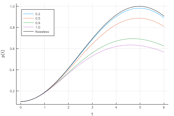
(p, t, pmax, tmax) = spatialsearch(psi0, Adjacency; kwargs...)

Example

This example reproduces (in a much less accurate way) part of Fig. 2 of the manuscript, where the probability as a function of time is shown for different values of the noise strength on the complete graph.

Here parallel evaluation is used with two worker process. Evaluating this script takes less than a minute on a laptop.

using Plots
using Distributed

addprocs(2)
@everywhere using QuantumSpatialSearch

N = 10; # Order of the graph
psi0 = superposition_state(N) # Initial state

# Noiseless spatial search
noiseless = spatialsearch(psi0, complete_graph_Ad; gamma=1. / N, time=6);

# Noise strength values
nus = [0.2, 0.5, 0.9, 1.0]

# Noisy spatial search simulation with 1000 noise realizations
noisy = [spatialsearch(psi0, complete_graph_Ad;
                    gamma=1. / N,
                    time=6,
                    mu=0.01,
                    noiseStrength=nu,
                    noiseRealizations=1000) for nu in nus]

# Plots
plot(noisy[1].t, [n.p for n in noisy],
                    label=nus,
                    xlabel="t",
                    ylabel="p(t)",
                    legend=:topleft)

plot!(noiseless.t, noiseless.p, c=:black, label="Noiseless")

mapleyustat/QuantumSpatialSearch