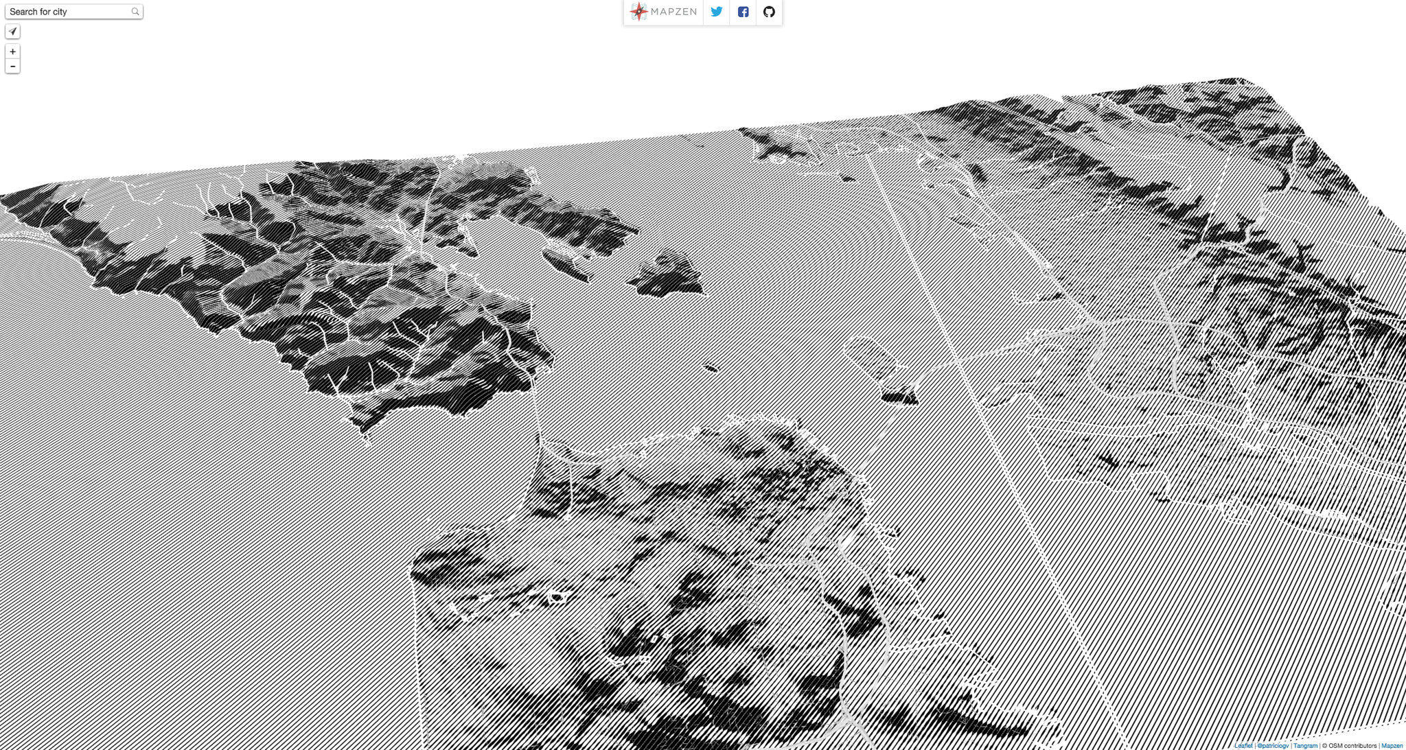
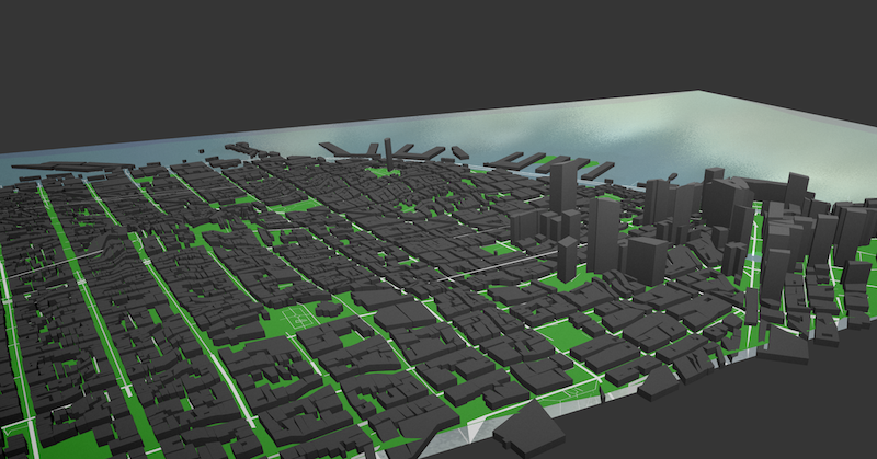
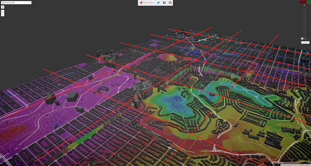
A series of experiments on terrain and elevation data for Tangram ignited by Patricio Gonzalez Vivo and powered by almost everybody in Mapzen
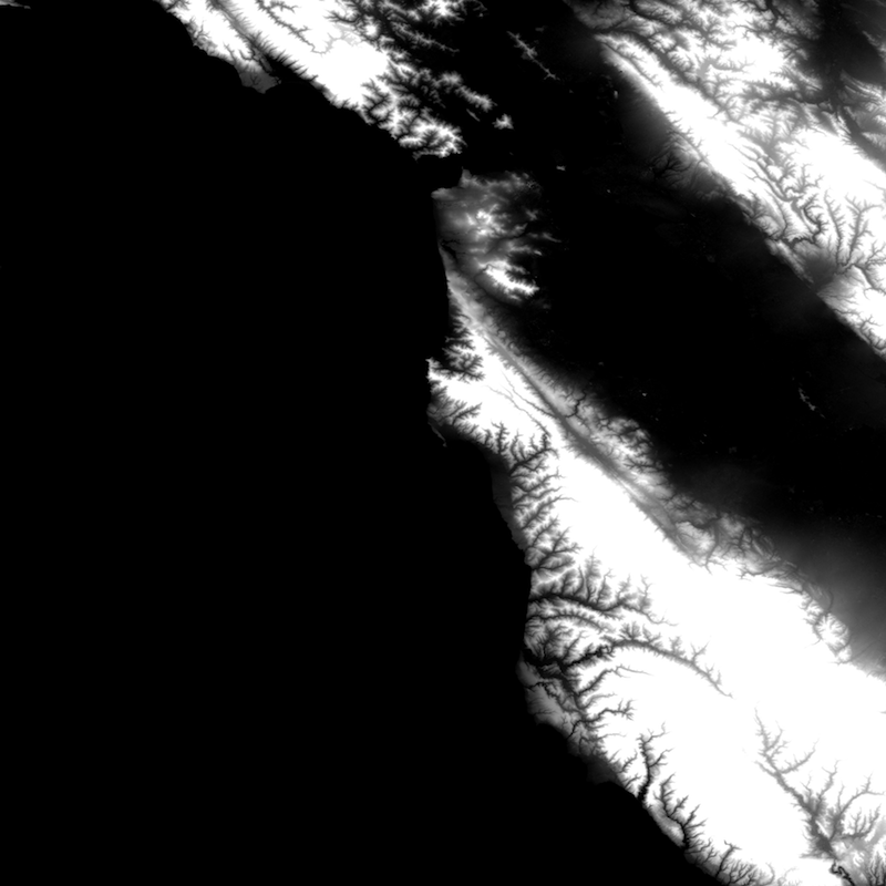
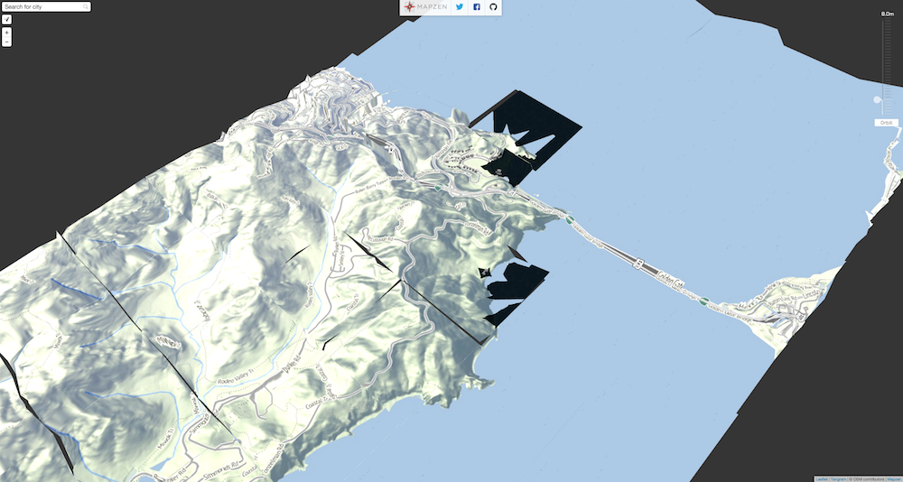
My first approach was to download a heightmap from the Shuttle Radar Topography Mission through Derek Watkins’s tool and simply project the vertices on the vertex shader.
After downloading and unzipping the tile from Shuttle Radar Topography Mission, I converted it to a PNG using gdal:
wget http://e4ftl01.cr.usgs.gov/SRTM/SRTMGL1.003/2000.02.11/N37W123.SRTMGL1.hgt.zip
tar xzvf N37W123.SRTMGL1.hgt.zip
gdal_translate -ot Int16 -of PNG N37W123.hgt N37W123.png
Downloading and inspecting the JSON file with the bounding boxes from Derek Watkins’s tool, I determine the boundaries of that tile. Which then I export to webmercator:
[-13692328.289900804, -13580946.954451224, 4439068.068371599, 4579465.0539420955]
Later I feed this values into a vertex shader on Mapzen’s Map Engine together with a MINZ and MAXZ for the elevation range:
geometry-terrain:
        animated: true
        mix: [generative-caustic, geometry-matrices, functions-map, filter-grain]
        shaders:
            uniforms:
                u_terrain: data/A/N37W123.png
                u_water_height: 0.
            defines:
                XMIN: -13692328.289900804
                XMAX: -13580946.954451224
                YMIN: 4439068.068371599
                YMAX: 4579465.0539420955
                ZMIN: -10.0
                ZMAX: 800.0
            blocks:
                global: |
                    bool inZone(vec2 _worldPos) {
                        return  _worldPos.x > XMIN && _worldPos.x < XMAX &&
                                _worldPos.y > YMIN && _worldPos.y < YMAX;
                    }

                    float getNormalHeight(vec2 position) {
                        vec2 worldPos = u_map_position.xy + position.xy;
                        if (inZone(worldPos)) {
                            vec2 st = vec2(0.0);
                            st.x = (worldPos.x-XMIN)/(XMAX-XMIN);
                            st.y = (worldPos.y-YMIN)/(YMAX-YMIN);
                            return texture2D(u_terrain, st).r;
                        } else {
                            return 1.1;
                        }
                    }

                    void extrudeTerrain(inout vec4 position) {
                        vec2 pos = position.xy;
                        float height = getNormalHeight(pos.xy);
                        if (height <= 1.0) {
                            position.z += ZMIN+height*(ZMAX-ZMIN);
                        }
                    }
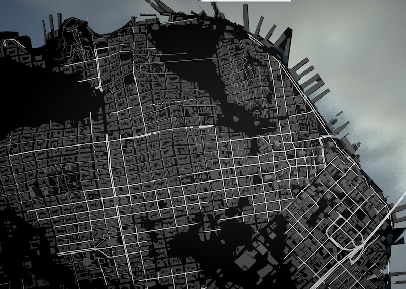
In the code above you can see how I’m checking if the vertex is inside the zone for where I have elevation data. If that’s true it extrudes the vertices.
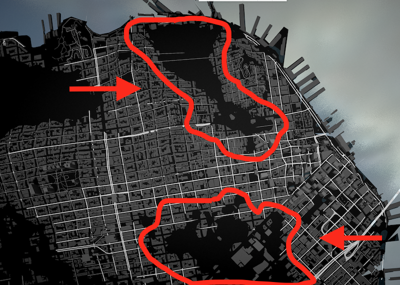
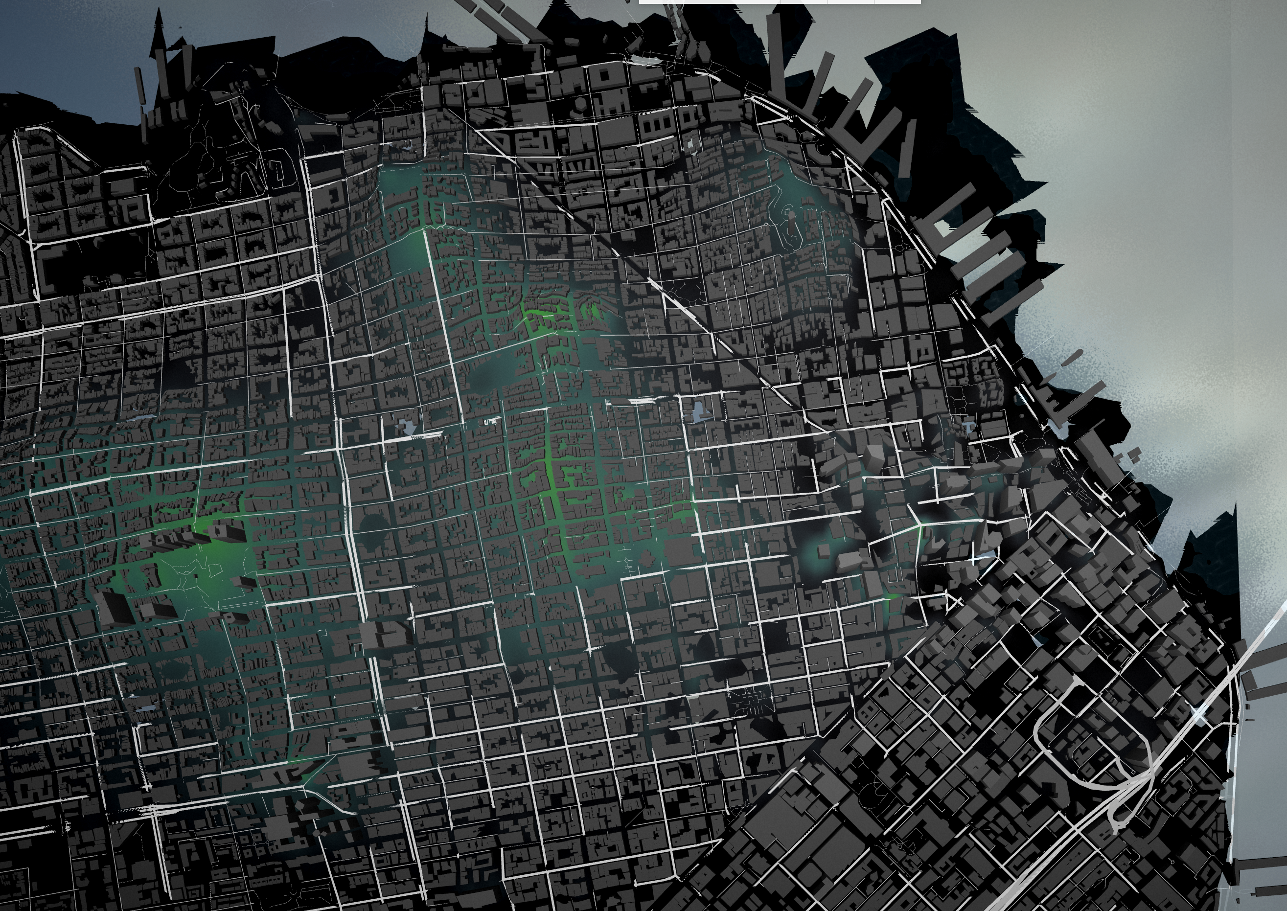
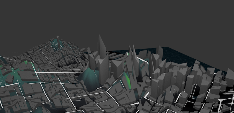
Sometimes the polygons that form the earth layer on OSM don’t have enough subdivisions and the vertices are extruded in a way that hides important features like roads and buildings, as seen in the image below.
To fix this I generate a custom set of plane tiles with subdivisions on important corners (coming from polygons and lines from OSM earth, roads and landuse layers)
By breaking the tiles into small fragments, the extrusion of the terrain doesn’t hide the geometry.
Running this script using the USGS ID (default: N37W123) and zoom levels (default: 3-17) will create the necessary tiles:
cd data
python makeATiles.py [USGS_ID] [ZOOM_RANGE]
Once the tiles are done and you look at the map in higher zoom levels, a new problem might emerge:
The top of the buildings have been extruded according to the heightmap, but in a incongruent way. To fix this issue we developed a new approach.
Data Sources:
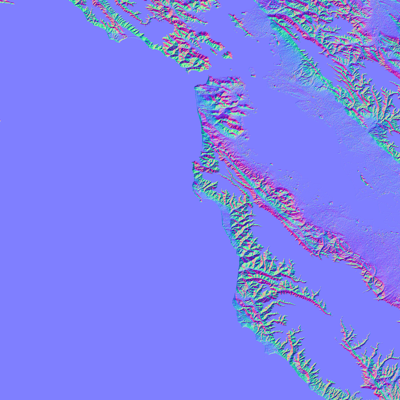
It is possible to illuminate the surface of the terrain by adding “normal” information to Tangram’s light engine. (The normal of a polygon is a three-dimensional vector describing the direction that it is considered to be facing, which affects the color and shininess of the polygon.)
We can make the NormalMap using the HeightMap we got from the Shuttle Radar Topography Mission using GIMP or the Tangram shader here using glslViewer like this:
cd data/
glslViewer normal.frag A/N37W123.png -o A/N37W123-normal.png
On the fragment shader we can use the following function to retrieve the normal values for each point…
vec3 getNormal(vec2 position) {
	vec2 worldPos = u_map_position.xy + position.xy;
	if (inZone(worldPos)) {
		vec2 st = vec2(0.0);
		st.x = (worldPos.x-XMIN)/(XMAX-XMIN);
		st.y = (worldPos.y-YMIN)/(YMAX-YMIN);
		return texture2D(u_normalmap, st).rgb*2.-1.;
	} else {
		return vec3(0.,0.,1.);
	}
}
and then use it on the YAML scene to modify the normals on the fragment shader:
	normal: |
		normal.gb = getNormal(v_orig_pos.xy);
Once the terrain is “lit”, the terrain looks like this:
Once I knew the lightening was right I try some non-realistic shading of it to understand better the use of this information:
Using the bounding box of the image we downloaded from Shuttle Radar Topography Mission](http://www2.jpl.nasa.gov/srtm/), I can construct a big rectangular polygon in which to draw the water level.
I use a Spherical Environmental Map on it together with some fragment shader code to disturb the normals using a regular simplex noise function to make it look more “natural”.
The code for this water is the following:
    water:
        base: polygons
        animated: true
        mix: [geometry-matrices, filter-grain]
        blend: inlay
        material:
            ambient: .7
            diffuse:
                texture: ../imgs/sem-sky-0001.jpg
                mapping: sphere map
        shaders:
            uniforms:
                u_offset: [0, 0]
                u_water_height: 0.
            blocks:
                position: |
                    position.z += u_water_height;
                    position.xyz = rotateX3D(abs(cos(u_offset.x))*1.3) * rotateZ3D(cos(u_offset.y)*1.57075) * position.xyz;
                normal: |
                    normal += snoise(vec3(worldPosition().xy*0.08,u_time*.5))*0.02;
                filter: |
                    color.a *= .9;
Then on the rest of the geometry I apply the following caustic filter to everything that above the water level.
        shaders:
            defines:
                TAU: 6.28318530718
                MAX_ITER: 3
            blocks:
                global: |
                    // Caustic effect from https://www.shadertoy.com/view/4ljXWh
                    vec3 caustic (vec2 uv) {
                        vec2 p = mod(uv*TAU, TAU)-250.0;
                        float time = u_time * .5+23.0;
                        vec2 i = vec2(p);
                        float c = 1.0;
                        float intent = .005;
                        for (int n = 0; n < int(MAX_ITER); n++) {
                            float t = time * (1.0 - (3.5 / float(n+1)));
                            i = p + vec2(cos(t - i.x) + sin(t + i.y), sin(t - i.y) + cos(t + i.x));
                            c += 1.0/length(vec2(p.x / (sin(i.x+t)/inten),p.y / (cos(i.y+t)/inten)));
                        }
                        c /= float(MAX_ITER);
                        c = 1.17-pow(c, 1.4);
                        vec3 color = vec3(pow(abs(c), 8.0));
                        color = clamp(color + vec3(0.0, 0.35, 0.5), 0.0, 1.0);
                        color = mix(color, vec3(1.0,1.0,1.0),0.3);
                        return color;
                    }

                filter: |
										vec2 wordPos = u_map_position.xy + v_orig_pos.xy;
                    if (inZone(wordPos) && ZMIN+height*(ZMAX-ZMIN)+worldPosition().z < u_water_height) {
                        color.gb += caustic(worldPosition().xy*0.005)*0.2;
                    }
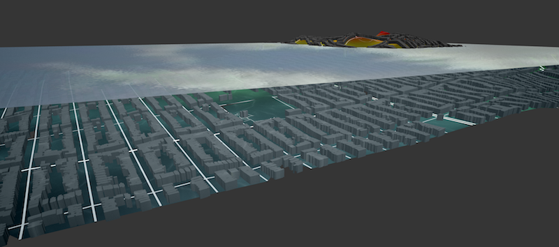
All of this makes the water looks like this:
This together with a slider updating the position of the uniform u_water_height allows a nice interactive animation of the sea levels rising:
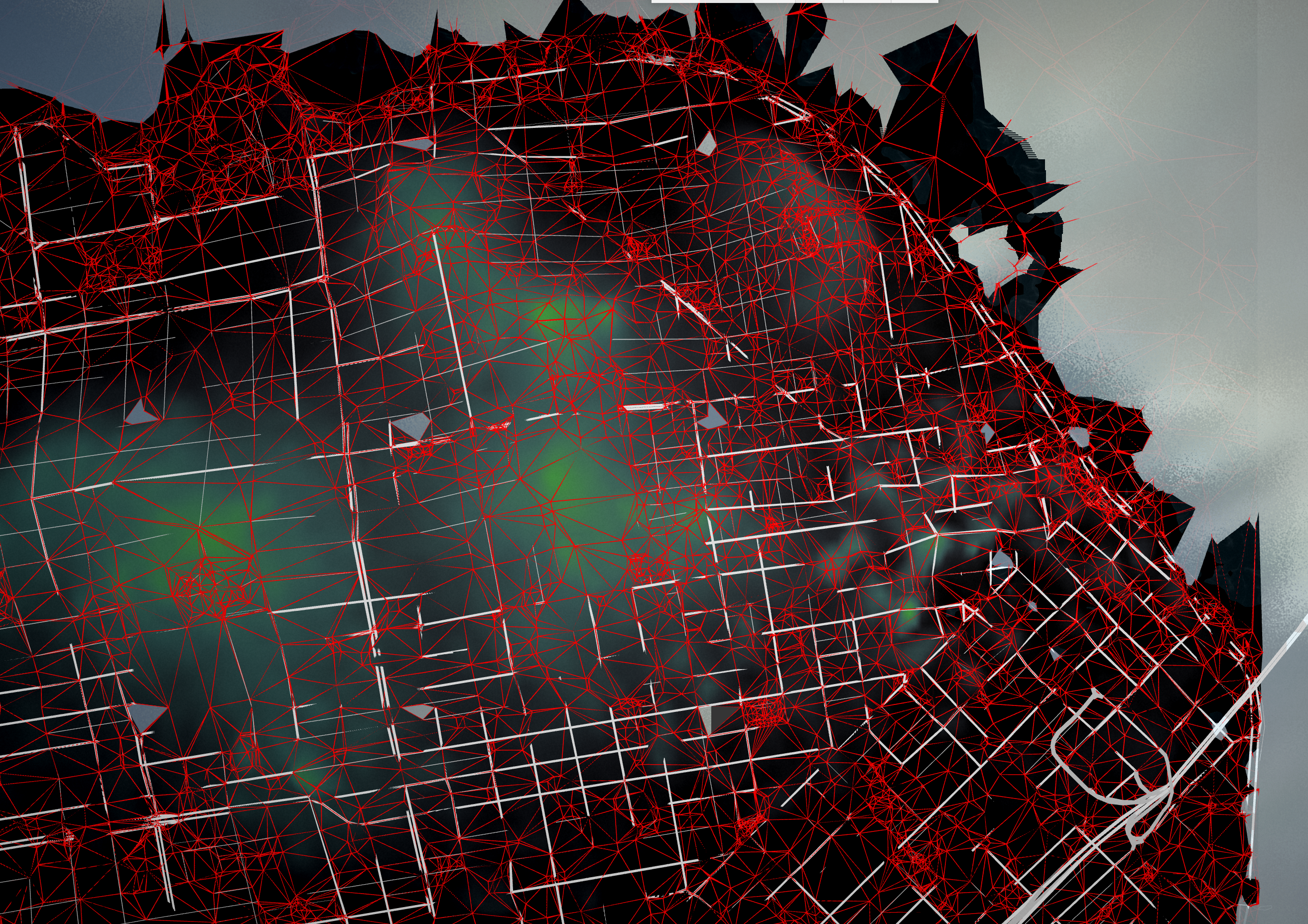
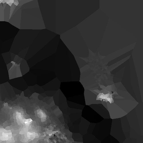
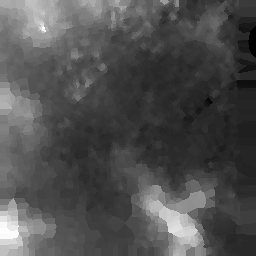
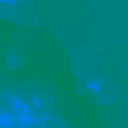
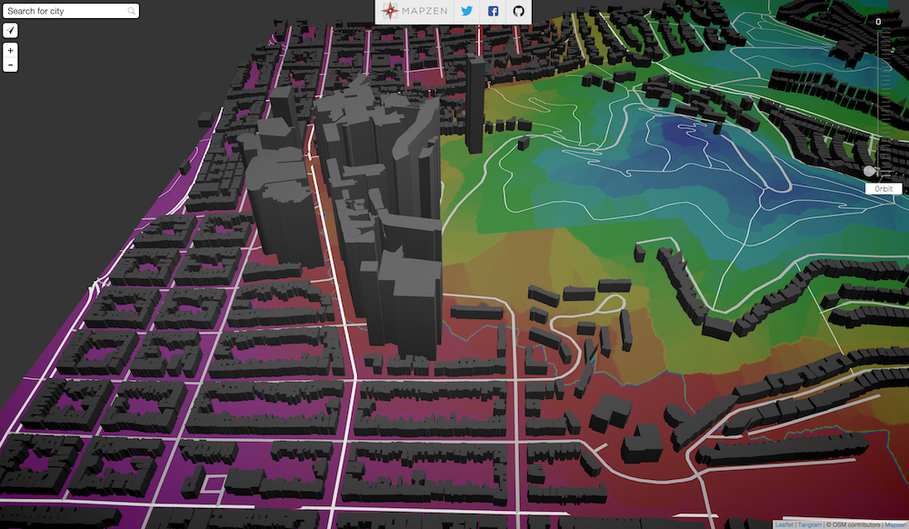
In order to solve the incongruence on building extrusion I thought it would be beneficial to have control over the heightmap. For that, we need to develop a new set of tiles. Each tile will have a double format of both GeoJSON and PNG images. The first will store the geometries explained on the previous section, plus the addition of building vertices, together with a PNG image that stores the elevation data in a useful and coherent way. For that I will fetch the elevation for just the present vertices using Mapzen’s elevation service and construct Voronoi tiled images from them.
The idea behind this approach is that vertices will fill ‘cells’ with a similar elevation. In the case of the buildings, all vertices should have the same height, and each cell of each corner will have the same value. This will work as a leveled “platform” for the building to rest upon, with out distorting the original roof elevation.
Because I’m composing the elevation images for each tile, we have way more control and curation of the data. This will allow us to increase the resolution and precision of the tile as we zoom in. But we still have another issue to resolve: Right now the elevation information is passed as a grayscale value, but the elevation range has to be hardcoded (look for ZMIN and ZMAX in the above code). If we are going to build tiles for the whole world we need a consistent way to pass this information rather than as a 1 bit value.
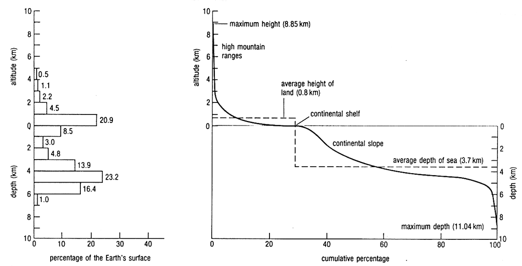
Checking with Kevin who is in charge of Mapzen’s elevation service, the elevation data have a precision of 2 bytes. A quick check on wikipedia reveals the highest and lowest points on earth.
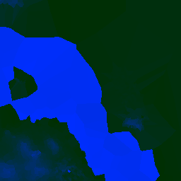
With an approximate range of -12000 to 9000 meters, color channels (GB = 255*255 = 65025) can accommodate this data range. The python script in charge of making the raster elevation tiles now looks like this...
	elev_unsigned = 12000+elevation
	GREEN = math.floor(elev_unsigned/255)%255
	BLUE = math.floor(elev_unsigned%255)
which produces a image that looks like this:
On the vertex shader we will need to “decode” this value:
	vec3 elev_color = texture2D(u_terrain, st).rgb;
	float height = -12000.0+elev_color.g*65025.+elev_color.b*255.;
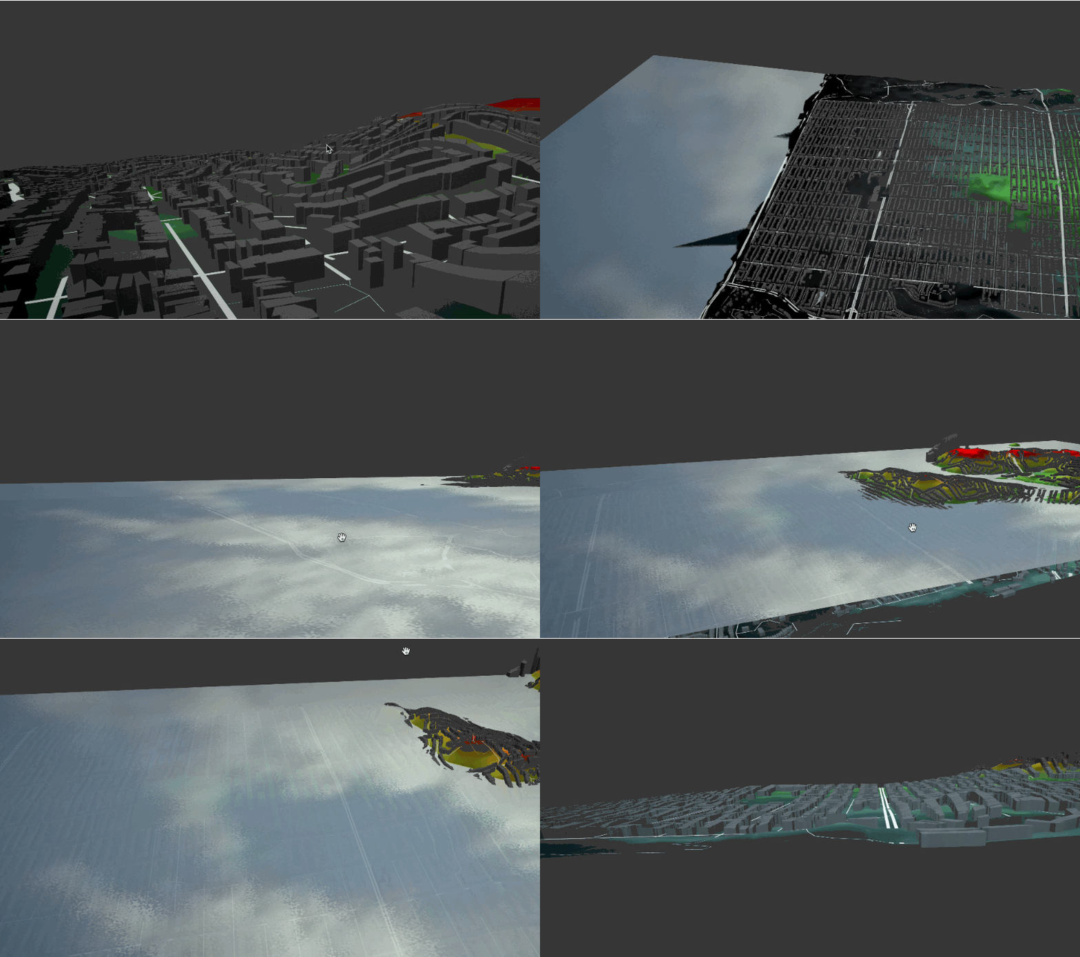
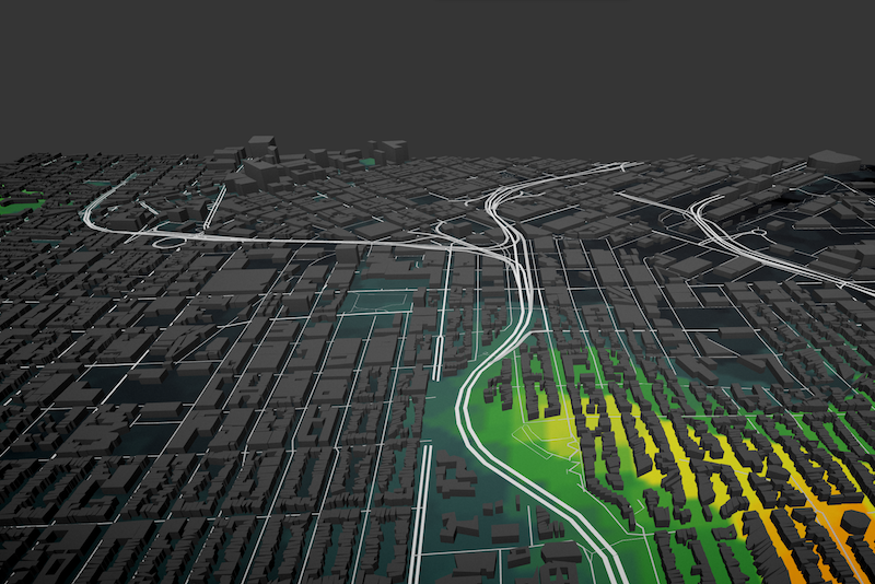
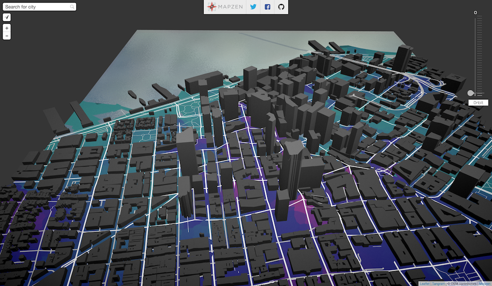
Putting it all together, each tile is rendered into something that looks like this!
The necessary tiles can be created by running the script with the OSM ID (default: 111968) and ZOOM RANGE (default: 3-17)
cd data
python makeATiles.py [OSM_ID] [ZOOM_RANGE]
Data Sources
Kevin Kreiser improve the voronoi algorithm to rasterize B tiles faster. In his own words, here is the comment on his PR:
so to properly display buildings without messing up their rooftops its nice to have an isoheight underneath them. @patriciogonzalezvivo added this by computing the brute force voronoi diagram where the cites were the building vertices, if i understand correctly. he mentioned though that the algorithm was very slow for complex scenes.
So here we let opencv do the heavy work. it has methods which likely use a variant of fortunes algorithm to compute the voronoi diagram (and its dual the delaunay triangulation) in O(nlogn) time. this is way faster than brute force.
another nice thing it does is allow us to rasterize the voronoi cells into a png fairly quickly. we do this by exploiting the fact that voronoi cells are always convex.
Kevin also suggest moving the offset to eliminate negative numbers to something that makes more sense than -12000 (the lower point on earth) to -32768. the half of the 16bits range. You can see this change here and here
Beside the significant increase in processing time, this changes made the B tiles more brighter and aquamarine blue, from that their current name Azulejos
I perform a “fast&dirty” modification to Tangram.js to load a textures per tile in a similar. Here is the commit to in src/scene.js and src/tile.js. Then by pointing to our tiles path in the yaml scene file:
 sources:
    ohm:
        type: TopoJSON
        url: //vector.mapzen.com/osm/all/{z}/{x}/{y}.topojson
    terrain:
        type: GeoJSON
        url: data/B/{z}-{x}-{y}.json
    elevation:
        type: Raster
        url: data/B/{z}-{x}-{y}.png
Tangram will create and download a texture per tile using that formula and pass it to the u_[raster_source_name] in this case u_elevation.
The GLSL Code in the style responsable for the extortion got way more clean and simplify:
	geometry-terrain:
        mix: [space-tile, generative-caustic, geometry-matrices, filter-grain]
        shaders:
            uniforms:
                u_elevation: elevation
                u_offset: [0, 0]
                u_water_height: 0.
            defines:
                    ZOFFSET: 0
            blocks:
                global: |
                    varying vec3 v_orig_pos;

                    float getHeight() {
                        vec3 color = texture2D(u_elevation, getTileCoords()).rgb;
                        if (color.rg != vec2(0.0)) {
                            return -32768.+color.g*65025.+color.b*255.;
                        } else {
                            return -1.0;
                        }
                    }

                    void extrudeTerrain(inout vec4 position) {
                        vec2 pos = position.xy;
                        float height = getHeight();
                        if (height != -1.0) {
                            position.z += height;
                        }
                    }
                position: |
                    position.z += ZOFFSET*u_meters_per_pixel;
                    v_orig_pos = position.xyz;
                    extrudeTerrain(position);
                    position.xyz = rotateX3D(abs(cos(u_offset.x))*1.3) * rotateZ3D(cos(u_offset.y)*1.57075) * position.xyz;
                color: |
                    float height = getHeight();
                    vec2 wordPos = u_map_position.xy + v_orig_pos.xy;
                filter: |
                    if (height+worldPosition().z < u_water_height) {
                        color.gb += caustic(worldPosition().xy*0.005)*0.2;
                    }
As you can see the on the above code now the shader only need tile coordinates (getTileCoords()) to get the right pixel on the texture. This is how it looks:
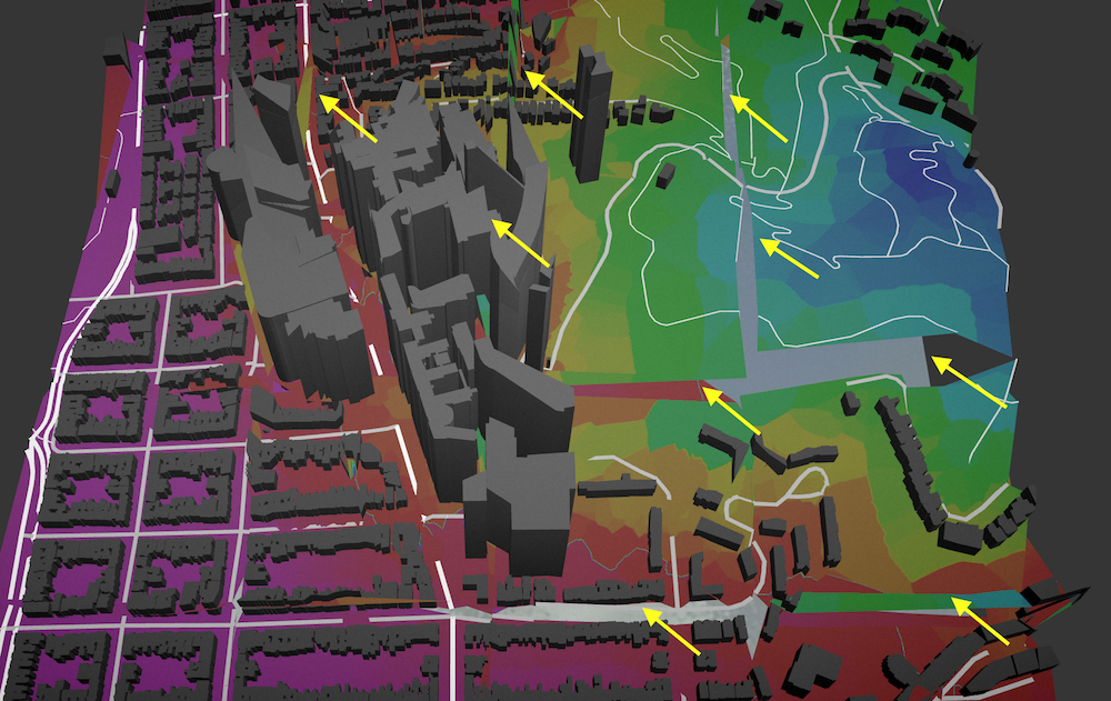
Unfortunately this progress also bring a new error to solve. Looking closely to the above image you can see some geometry been erroneously extrude close to tile edges
This seams to be cause because building vertices tend to exceed the limits of a tile. Once this data is provide to the tile and process by the shader, probably is not finding information outside the tile edges.
Also it seams to be having the opposite problem when there is no vertices close enough to the edges.
For the next round of exploration I will consult with Rob Marianski how to only use the vertices inside a tile and add extra once to fill the spaces.
Taking advantage of the changes made on Tangram to load raster tiles as per tile textures, is easy to use this images to shade the terrain.
sources:
		…
    stamen:
        type: Raster
        url: http://spaceclaw.stamen.com/terrain/{z}/{x}/{y}.png
…
styles:
		…
    elevate_ls:
        base: polygons
        mix: [geometry-terrain]
        shaders:
            defines:
                    ZOFFSET: -1
            blocks:
                color: |
color.gb = texture2D(u_stamen, getTileCoords()).rgb;Today I spend some time to make a script to automatically install the linux packages and python modules:
-
PIL
sudo pip install pilsudo pip install requests- NumPy:
sudo pip install bumpy- OpenCV for python:
sudo apt-get install python-opencv- Shapely:
sudo apt-get install libgeos++
sudo pip install shapely
Now using the script install.sh I can replicate what was working on my Raspberry Pi to any other linux machine :)
Finally fixed the tile-edge glitch which was made by two different reasons. There was extra geometry been constructed from building vertices outside the tile boundaries, and a problem with the modelPosition() output on getTileCoords(). Now that module looks like this:
styles:
		…
    space-tile:
        shaders:
            blocks:
                global: |
                    // Variant to be add to both vertex and fragments shaders
                    varying vec3 v_pos;
                    //
                    // Get the coordinates in tile space
                    // ================================
                    vec2 getTileCoords() {
                        return vec2(v_pos.x, 1.+v_pos.y);
                    }

                position: |
                    // Normalize the attribute position of a vertex
                    v_pos = modelPosition().xyz;
		…
Previously the presence of a fract() function was wrapping around what seams to be negative values from modelPosition().y.
Now tiles stitch perfectly between each other:
And finally we can appreciate building with flat roofs.
Terrain geometry tiles (.json files on data/B folder) had more precession than the raster elevation image (.png files on data/B folder). By downsampling the precession of the computed vertices to the same as the raster image (255x255) we save almost 50% on critical tiles. For example tile 9-82-198.json use to compute 30,663 vertices into 42,008 triangles producing a TopoJSON file of 28.5MB. After the simplification the total amount of triangles go reduce to 22.468, which means 17.2 MB.
This number still is very big, so I will keep researching ways to reduce the number of triangles with out reducing visual artifacts or degenerated geometry.
-
Instad of re use the terrain geometry for the water, make a big big tile of the size of the hole earth to draw less triangles
-
Make shaders more efficient: probably take out noise and fbm functions for grain effect and stuff.
-
Make geometry more efficient: Under zoom level 12, geoJSON tiles are too big (~10mb in the worst scenario). These zoom levels may not need so much definition for the terrain geometry. Simplifying data coming from elevation contours and heightmap/normalmap may be enough. Contour/roads data is enough until between 1-14 as the buildings are too small to be visible. Or maybe just heightmap/normalmap is enough as users don’t really see the terrain under 12.
-
Add more vertices to compute on the GeoJson geometry tiles using contour data, so we are sure there is enough information to cover non urban areas.
-
Solve over drawing
cd ~
git clone —depth 1 https://github.com/mapzen/terrarium.git
cd terrarium
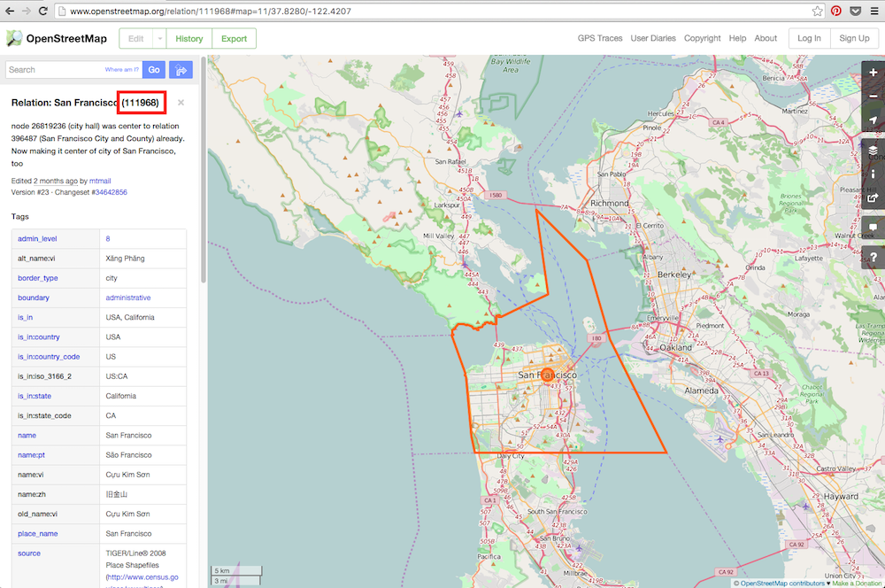
./install.shmakeBTiles.py require a OSM ID of the place you want to make tiles for it. To get this id go to openStreetMap and type the name of a city, and search for the number between ( ).
Then pass this number as the first argument of the script, while the third argument is the range of zoom you are interested
cd data
python makeBTiles.py 111968 3-17-
Patricio Gonzalez Vivo: Came up with the first round of A and B tiles ideas
-
Kevin Kreiser: improve the voronoi algorithm to rasterize B tiles faster
-
Rob Marianski: help us with his python tiling magic
