How to solve nonlinear optimization problems using different solvers and techniques based on Python.
Author
Marcel Cases i Freixenet <marcel.cases@estudiantat.upc.edu>
Course
Topics on Optimization and Machine Learning (TOML-MIRI)
FIB - Universitat Politècnica de Catalunya. BarcelonaTech
April 2021
Considering the optimization problem:
minimize
ex1(4x12 + 2x22 + 4x1x2 + 2x2 + 1)
subject to
x1x2 - x1 - x2 ≤ -1.5
-x1x2 ≤ 10
var
x1, x2
This is not a convex optimization problem. There are different local and global optimizaiton points.
Solutions obtained with Scipy's optimize.minimize library, using SLSQP (Sequential Least Squares Programming) method:
| Initial point x0 | Optimal p* | Coordinates (x1, x2)* | Function evaluations (nfev) | Execution time (ms) |
|---|---|---|---|---|
| (0,0) | 0.0235 | (-9.54,1.04) | 54 | 7.99 |
| (10,20) | 3.0607 | (1.18,-1.73) | 70 | 11.00 |
| (-10,1) | 0.0235 | (-9.54,1.04) | 34 | 5.98 |
| (-30,-30) | 0.0235 | (-9.54,1.04) | 41 | 7.97 |
Solutions using the same parameters, plus a Jacobian input:
| Initial point x0 | Optimal p* | Coordinates (x1, x2)* | Jacobian evaluations (njev) | Execution time (ms) |
|---|---|---|---|---|
| (0,0) | 0.0235 | (-9.54,1.04) | 17 | 52.02 |
| (10,20) | 3.0607 | (1.18,-1.73) | 21 | 65.02 |
| (-10,1) | 0.0235 | (-9.54,1.04) | 11 | 28.02 |
| (-30,-30) | 141.0364 | (-1.06,-6.45) | 21 | 60.99 |
As shown in the tables, different initial points converge to different optimal solutions. When Jacobian is introduced, there is one new result 141.0364 which is far from the other optimals.
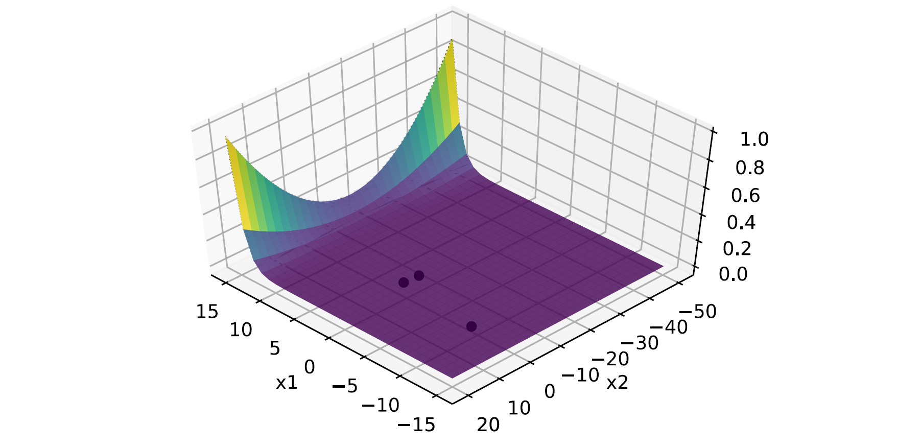
The plot of the objective function as well as the optimal points is as follows:
For this example, the graph does not help much to understand the problem because it is quite difficult to identify visually the minimum points, and the constraints are not visible.
Considering the optimization problem:
minimize
x12 + x22
subject to
-x1 ≤ -0.5
-x1 - x2 + 1 ≤ 0
-x12 - x22 + 1 ≤ 0
-9x12 - x22 + 9 ≤ 0
-x12 - x2 ≤ 0
x1 - x22 ≤ 0
var
x1, x2
The objective function is convex but some constraints are not, e.g., -x12 - x22 + 1 ≤ 0, which is a set with an empty circle. Thus, this is not a convex optimization problem.
Testing with different initial points x0 and SLSQP method on Scipy,
- (x1, x2) = (10, 10) is a feasible initial point, and returns the results:
- Optimal p* = 2.0
- Coordinates (x1, x2) = (1.0, 1.0)
- (x1, x2) = (0, 0) is a non-feasible initial point. The solver threw the message
Positive directional derivative for linesearch, meaning that the optimizer got into a position where it did not manage to find a direction where the value of the objective function decreases.
After running the solver with the Jacobian input and the feasible initial point above, the obtained results were the same, with just 9 Jacobian evaluations njev and 40.96ms, as compared to 73 function evaluations nfev and 25.06ms without the Jacobian method.
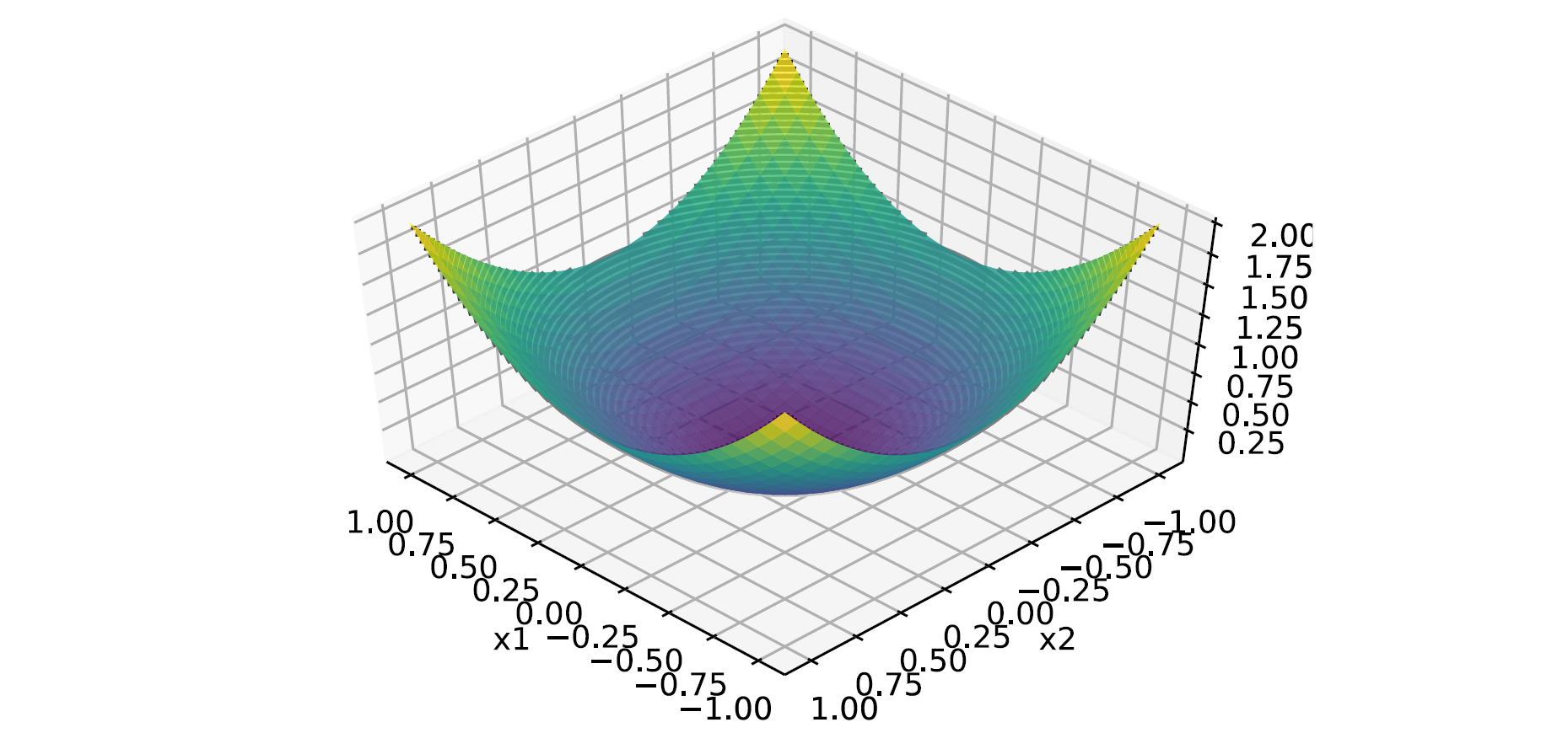
The plot of the objective function is as follows:
Considering the optimization problem:
minimize
x12 + x22
subject to
x12 + x1x2 + x22 ≤ 3
3x1 + 2x2 ≥ 3
var
x1, x2
It is a convex optimization problem. The objective function as well as all the constraints are convex.
Two different solvers have been used to obtain the optimal:
- Scipy's
optimize.minimizelibrary, using SLSQP and the combinations:- bare solver
- Jacobian as an input
- Jacobian and Hessian as an input
- CVXPY
Using (x1, x2) = (10, 10) as the initial guess, results are the following:
| Solver | Optimal p* | Coordinates (x1, x2)* | Iterations | Execution time (ms) |
|---|---|---|---|---|
| Scipy | 0.6923 | (0.6923, 0.4615) | 12 | 5.01 |
| Scipy with Jacobian | 0.6923 | (0.6923, 0.4615) | 4 | 16.92 |
| Scipy with Jacobian and Hessian | 0.6923 | (0.6923, 0.4615) | 4 | 17.99 |
| CVXPY | 0.6923 | (0.6923, 0.4615) | not provided | 33.35 |
Four initial points x0 have been tested [(10, 10), (-10, 10), (10, -10), (-10, -10)], and all of them converge to the same optimal result.
CVXPY also provides the dual values λ1 = 0 and λ2 = 0.4615.
Considering the optimization problem:
minimize
x2 + 1
subject to
(x-2)(x-4) ≤ 0
var
x
Using CVXPY as the solver, the following results are obtained:
solve 4.999999979918552
status: optimal
optimal value p* =  4.999999979918552
optimal var: x =  [2.]
optimal dual variables lambda =  [2.00003221]
exec time (ms):  13.0
Using Scipy's optimize.minimize with Jacobian and Hessian as the solver, the following results are obtained:
     fun: array([5.])
     jac: array([4.])
 message: 'Optimization terminated successfully'
    nfev: 8
     nit: 7
    njev: 7
  status: 0
 success: True
       x: array([2.])
JAC+HESS: optimal value p* [5.]
JAC+HESS: optimal var: x =  [2.]
exec time (ms):  24.9931640625
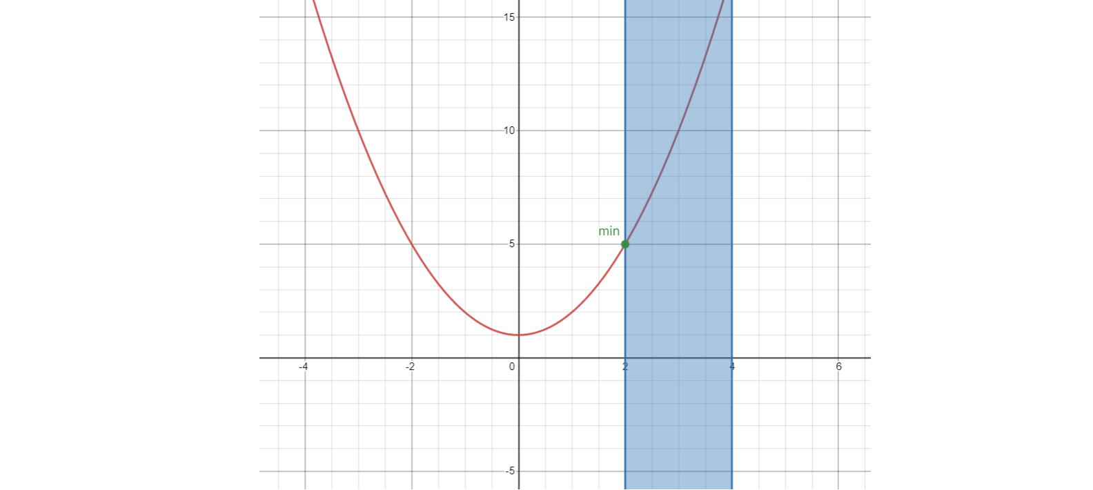
Graphically,
As shown in the plot, the minimum of the function within the feasible area is the point (x*, p*) = (2.0, 5.0). The function is convex in all its domain. Both solvers converge to the same result.
The dual values obtained are λ = 2 and d*=5.
Considering the optimization problem:
minimize
x12 + x22
subject to
(x1 - 1)2 + (x2 - 1)2 ≤ 1
(x1 - 1)2 + (x2 + 1)2 ≤ 1
var
x1, x2
Using CVXPY as the solver, the following results are obtained:
solve 0.9999658242523712
status: optimal
optimal value p* =  0.9999658242523712
optimal var: x1 =  0.9999802295393706  x2 =  1.9912424211981957e-14
optimal dual variables lambda1 =  28013.52446782075
optimal dual variables lambda2 =  28013.52446781738
The Lagrange multipliers do exist for this optimization problem, although they have a large value
Gradient Descent Methods for an unconstrained optimization problem
The Gradient Descent Algorithm assumes that
x(k+1) = x(k) + tΔx = x(k) - t∇f(x(k))
For this problem, two functions are minimized:
- f(x) = 2x2 - 0.5, with initial point x0 = 3
- f(x) = 2x4 - 4x2 + x - 0.5, with initial points x0 = -2, x0 = -0.5, x0 = 0.5, x0 = 2
Two Gradient Descent methods are used:
- Backtracking Line Search
- Newton’s Method
This problem has been solved by using a custom developed solver for BLS, with basic Python libraries; and Scipy for Newton's.
Backtracking Line Search algorithm
def backtrack(dfx, x0, step):
    incumbent = x0 # result
    iters = 0
    acc = 1
    while (acc >= 1e-4):
        newincumbent = incumbent - step*dfx(incumbent)
        acc = np.absolute(newincumbent - incumbent)
        incumbent = newincumbent
        iters += 1
    return incumbent, iters, acc, step
The inputs of the function are the first-degree derivative of the objective function dfx, an initial point x0, and a step that sets the resolution of the solver. The solver iterates indefinitely until the accuracy value acc is reached, which means that a local/global minima has been found. After this, the solution (x*) is returned (incumbent), as well as the number of iterations, the accuracy and the step value.
Newton’s Method algorithm
Newton's Method uses a second-order Taylor series expansion of the function about the current design point, i.e. a quadratic model. Scipy's library optimize uses this method for computing the minimum value of the function.
Results and performance
For f(x) = 2x2 - 0.5, with initial point x0 = 3, the results obtained with both methods are the following:
| Solver | Optimal p* | Optimal x* | Iterations | Execution time (ms) |
|---|---|---|---|---|
| Backtracking Line Search | -0.498 | 0.0248 | 1196 | 1982.93 |
| Newton's with Jacobian and Hessian | -0.5 | 0.0 | 5 | 9.00 |
For f(x) = 2x4 - 4x2 + x - 0.5, the results obtained with both methods are the following:
| Initial point x0 | Solver | Optimal p* | Optimal x* | Iterations | Execution time (ms) |
|---|---|---|---|---|---|
| -2 | Backtracking Line Search | -3.529 | -1.062 | 228 | 374.25 |
| -2 | Newton's with Jacobian and Hessian | -3.529 | -1.057 | 7 | 15.99 |
| -0.5 | Backtracking Line Search | -3.529 | -1.052 | 304 | 476.43 |
| -0.5 | Newton's with Jacobian and Hessian | -3.529 | -1.057 | 8 | 18.02 |
| 0.5 | Backtracking Line Search | -1.533 | 0.922 | 399 | 641.96 |
| 0.5 | Newton's with Jacobian and Hessian | -1.533 | 0.930 | 8 | 18.02 |
| 2 | Backtracking Line Search | -1.533 | 0.937 | 297 | 485.86 |
| 2 | Newton's with Jacobian and Hessian | -1.533 | 0.930 | 7 | 16.00 |
For the BLS, the step parameter has been set to 1e-3. Making it lower will improve the performance of the algorithm by reducing the computing time, but the results would not be as thorough. The accuracy (which is also the stop criteria, as specified in the statement) has been set to 1e-4.
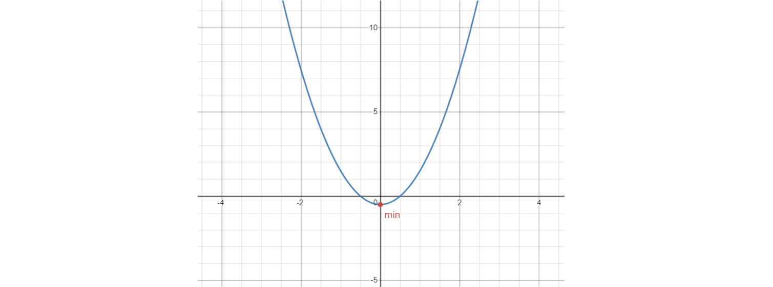
Plots
For f(x) = 2x2 - 0.5, there is a convex function. Any initial point will converge to the global minimum of the function, which is (x*, p*) = (0.0, -0.5).
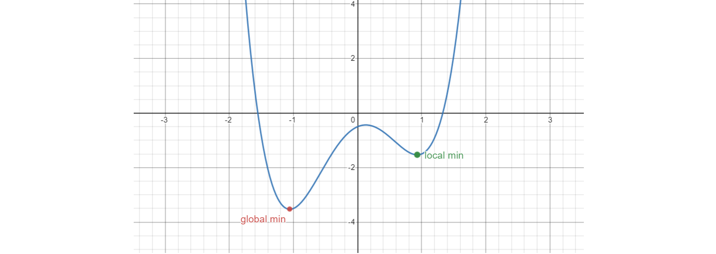
For f(x) = 2x4 - 4x2 + x - 0.5, there is a non-convex function. Depending on the initial point, the solution will fall into either:
- the local minima, if x0 > ~0.15
- the global minima, otherwise
The local minima is (x*, p*) = (0.92, -1.53), and the global minima is (x*, p*) = (-1.05, -3.52).
Network Utility problem
A networking problem where sources traverse links from routers in order to transmit data. Source 1 traverses link 1 and 2, source 2 traverses link 2 and source 3 traverses link 1 and 5. The goal is to maximize the transmission rate xs.
The model of the problem is the following:
maximize
log x1 + log x2 + log x3
subject to
x1 + x3 ≤ 1
x1 + x2 ≤ 2
x3 ≤ 1
x1, x2, x3 ≥ 0
var
x1, x2, x3
The original problem can be expressed as a logarithmic sum, which makes it convex. Using CVXPY as the solver, the following results are obtained:
solve -0.9547712365062518
status: optimal
optimal value p* = -0.9547712365062518
optimal var: x1 = 0.4226489442893967  x2 = 1.577351049782123  x3 = 0.5773510541368012
optimal dual variables lambda1 = 1.7320483134403175
                        lambda2 = 0.6339745314617544
                        lambda3 = 6.437850296384749e-09
                        lambda4 = 6.544679319172325e-09
                        lambda5 = 1.7755538040590713e-09
Resource Allocation problem
A resource allocation problem for a wireless network where traffic has to be assigned to nodes and links. Collisions have to be avoided (e.g. time R12 can not transmit simultaneously with R23), and links are bidirectional (R12 + R23 + R32 ≤ 1).
The model of the problem is the following:
maximize
log x1 + log x2 + log x3
subject to
x1 + x2 ≤ R12
x1 ≤ R23
x3 ≤ R32
R12 + R23 + R32 ≤ 1
xi, Ri ≥ 0
var
x1, x2, x3, R12, R23, R32
It can be expressed as a convex problem as well. Using CVXPY as the solver, the following results are obtained:
solve -3.9889840093737394
status: optimal
optimal value p* = -3.9889840093737394
optimal var: x1 = [0.16666665]  x2 = [0.33333335]  x3 = [0.33333335]
                        r12 = [0.5]  r23 = [0.16666665]  r32 = [0.33333335]
optimal dual variables lambda1 = [2.99999975]   lambda2 = [2.99999975]
                        lambda3 = [2.99999975]   u1 = [2.99999975]
Class slides
CVXPY https://www.cvxpy.org/
Convex optimization https://en.wikipedia.org/wiki/Convex_optimization
Lagrangian Duality and Convex Optimization https://www.youtube.com/watch?v=thuYiebq1cE
Sequential Least Squares Programming https://en.wikipedia.org/wiki/Sequential_quadratic_programming
Backtracking Line Search https://sites.math.washington.edu/~burke/crs/408/lectures/L7-line-search.pdf
Quadratic Programming with Python and CVXOPT https://courses.csail.mit.edu/6.867/wiki/images/a/a7/Qp-cvxopt.pdf
