This is a R package developed to design and simulate formal Chemical Reaction Networks (CRN) and DNA-based reaction networks using Strand Displacement reactions.
The theoretical field of Chemical Kinetics has developed brightly the last years, being capable of design many circuits and algorithms (such as the Message Passing Inference [2] and a Least mean Squares Estimator [3]) using CRNs as a building block. CRNs are formed by reactions as:
A + B -> C,
where the species A combined with the species B results in the species C
(a species can be a molecule of a chemical element or compound). The reaction
also has a velocity related to it (how fast the reactants are consumed to
generate the products).
The problem is: what chemical elements can be used to interact the way as specified and with the velocity desired? There is where the DNA comes in to play.
DNA are very versatile molecule structures. A B can be DNA complexes
designed to interact to each other in a certain way to produce another complex
or strand C in a certain velocity, or even interact with another chemical
entities to generate high fluorescence, for example (as a debugging mechanism
or strategy to get a response from the CRN execution) [4].
To ‘compile’ a formal CRN into a DNA-based one, a translation schema must be
followed. The one used in the project is described by Soloveichik et al.
[1]. Others can be implemented in a modular manner and simulated using
the simulation functions of DNAr explained later on.
This package simulates Formal CRNs and DNA-based CRNs using a system of ODEs (Ordinary Differential Equations) which describe the CRN's behavior through time. This is a simplified simulation approach since it does not considered unintended/leaked reactions and other real-word aspects, but it's still useful to rapidly verify if a CRN can behaves as expected in a fully-controlled scenario.
Main functions and their description
| Description | Code Function |
|---|---|
| Simulate a formal CRN | react() |
| Generate and simulate a DNA-based CRN according to the approach [1] | react_4domain() |
| Analyze the Ordinary Differential Equations (ODEs) used to simulate the CRN | analyze_behavior() and eval_derivative() |
| Compare the behavior of species. Useful to track the changes of the CRN’s behavior after a change of parameters | compare_behaviors_nrmse() |
| See, export and import the behavior of a simulated CRN | plot_behavior(), save_behavior_csv(), load_behavior_csv() |
| Export the DNA-based CRN generated to the Microsoft Visual DSD (for a further in-depth simulation) | save_dsd_script() |
All the functions are documented and it can be accessed by typing
?<function-name> in the R console (after loading the package).
Example: ?react.
If you want to quickly try-out that CRN presented in a paper, or check if an idea that you have about cyclic reaction can work using DNA, or even tweak a CRN with new parameter values and reactions and see if it works, this is the package for you. 👍
DNAr is designed to be simple to use and give you initial information about a CRN (formal and DNA-based) and help you understand how it works (or why it doesn't) by allowing fast and easy (and simplified) simulations. It is not a package to simulate CRNs in depth, analyze leakage or potential unwanted reactions, nor to verify the suitability of a CRN for a real-world scenario.
Firstly, using the R console, install the devtools package:
install.packages("devtools")After that, just install the DNAr package:
library(devtools)
devtools::install_github('DanielKneipp/DNAr')Let’s take a look at the reaction A --k--> B, for example. Defining the
initial conditions as follows:
[A]_0 = 1E-5 M(Initial concentration ofA);[B]_0 = 0 M;- rate constant (
k) of5E-5 1/s; - time period of 72,000 seconds,
we would have the following code to simulate it:
library(DNAr)  # Loading the library

# Simulating
b <- react(
    species   = c('A', 'B'),
    ci        = c(1e-5, 0),
    reactions = c('A -> B'),
    ki        = c(5e-5),
    t         = seq(0, 72000, length.out = 10)  # Using 10 time points
)
Firstly, the name of the species and their initial concentrations are defined (following the same order). Then, the reactions and their ration constants are specified (also following the same order). Finally, the time period is defined by given its range and the number of points to process (more points mean more accurate and time-consuming simulations)
All the simulated behavior is held by the b variable. By typing b in the
console you can see the variation of the concentrations throughout time.
> b
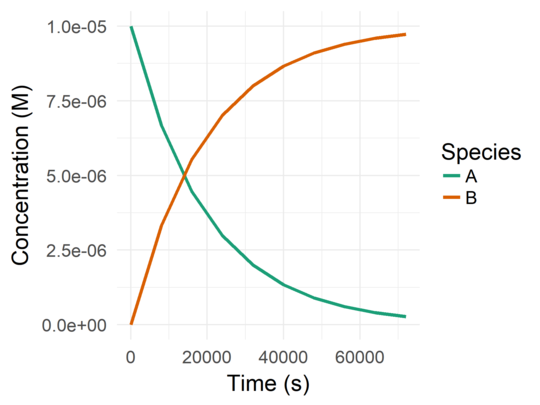
    time            A            B
1      0 1.000000e-05 0.000000e+00
2   8000 6.671976e-06 3.328024e-06
3  16000 4.462676e-06 5.537324e-06
4  24000 2.990997e-06 7.009003e-06
5  32000 2.004515e-06 7.995485e-06
6  40000 1.343019e-06 8.656981e-06
7  48000 8.997926e-07 9.100207e-06
8  56000 6.028607e-07 9.397139e-06
9  64000 4.039198e-07 9.596080e-06
10 72000 2.706274e-07 9.729373e-06
To plot the result, just do:
plot_behavior(
    b,
    x_label     = 'Time (s)',
    y_label     = 'Concentration (M)',
    legend_name = 'Species'
)
This code will yield the following plot:
To see more examples with multiple reactions, just type ?react in the
R console.
To generate and simulate a DNA-based CRN, the function called react_4domain()
is used. A few more parameters must be defined in contrast to react().
The parameters used to simulate a formal CRN remains the same. species, ci,
reactions, ki and t should be defined exactly like a formal CRN. qmax,
cmax, alpha and beta are new parameters which must be specified following
the guidelines described by [1].
The react_4domain() will automatically generate a DNA-based CRN correspondent
to the formal CRN specified (following the approach [1]) and simulated it.
As an example, let's simulate the reaction A + B --> C.
r <- react_4domain(
    species   = c('A', 'B', 'C'),
    ci        = c(1e-6, 1e-6, 0),
    reactions = c('A + B -> C'),
    ki        = c(1e2),
    qmax      = 1e6, cmax = 1e-4,
    alpha     = 1,   beta = 1,
    t         = seq(0, 72000, length.out = 10)
)
r holds information about the CRN that was actually simulated (the DNA-based
one) and the behavior obtained from it. These are the attributes of r:
| Attribute | Description |
|---|---|
r$behavior |
The behavior of the DNA-based CRN (like the data table returned by react()) |
r$species, r$ci, r$reactions and r$ki |
The DNA-based CRN with its parameters (used to simulate it with react()) |
By typing r$reactions, you can see the DNA reactions used to emulate the
behavior of the formal CRN (A + B -> C in this case).
> r$reactions
[1] "A + L1 --> H1 + W1"    "H1 + W1 --> A + L1"    "B + H1 --> O1"    "O1 + T1 -->  C"
Notice that these reactions are the same as the ones shown in the Figure 3 from
[1], where A = X_1, B = X_2, C = X_3 and W1 = B_i.
The initial concentrations of the species and the rate constant of the reactions also can changed. However, the overall behavior of the formal species in the DNA-based CRN should be quite similar to the formal one.
To plot the results, the same plot_behavior() function can be used:
plot_behavior(
    r$behavior,
    x_label            = 'Time (s)',
    y_label            = 'Concentration (M)',
    legend_name        = 'Species',
    species            = c('A', 'B', 'C'),
    variable_line_type = TRUE
)
Note that a species parameter is now being specified. This selects the
species to be plotted. If you want to see the behavior of all the auxiliary
species, just remove this parameter definition.
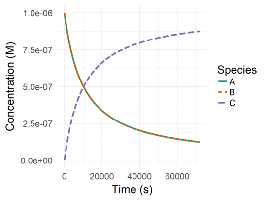
The species A and B will have the same behavior. To allow us to both species
in the plot, the parameter variable_line_type is set to TRUE, making the line
types vary according to the species.
This code will yield the following result:
In order to simplify the process of analyze and understand the behavior of a
CRN, analyze_behavior() shows the derivatives used for the simulation. Given
the CRN parameters, it returns the derivatives for each species.
d <- analyze_behavior(
    species   = c('A', 'B', 'C'),
    ci        = c(1e-5, 0, 1e-8),
    reactions = c('A -> B',
                  'A -> C'),
    ki        = c(5e-5,
                  3e-5)
)
> d['A']
A
1 d[A]/dt = (-5e-05 * [A]) + (-3e-05 * [A])You also can pass the behavior to it allowing you to analyze the values
of each derivative variables in selected points in time. In the following code
the derivate of A is shown at initial conditions.
b <- react(
    species   = c('A', 'B', 'C'),
    ci        = c(1e-5, 0, 1e-8),
    reactions = c('A -> B',
                  'A -> C'),
    ki        = c(5e-5,
                  3e-5),
    t         = seq(0, 72000, length.out = 10)
)

d <- analyze_behavior(
    species     = c('A', 'B', 'C'),
    ci          = c(1e-5, 0, 1e-8),
    reactions   = c('A -> B',
                    'A -> C'),
    ki          = c(5e-5,
                    3e-5),
    behavior    = b,
    time_points = c(1) # Selecting the first time point
)
> d['A']
A
1 d[A]/dt = (-5e-05 * 1e-05[A]) + (-3e-05 * 1e-05[A])Now you can see the concentration of A at initial conditions (alongside each
[A]).
To see if the concentration of A will decrease or increase at this time point,
just evaluate the derivative with:
> eval_derivative(d['A'])
[1] -8e-10
The resultant signal shows if [A] will increase or decrease (decrease in this
case), and the absolute value indicates the rate of change.
To better understand why the derivative of A has this value,
eval_derivative_part() can be used to evaluate each parenthesis of
the derivative separately. This will indicate how each reaction that interacts
with A is contributing to that value.
> eval_derivative_part(d['A'])
(-5e-05 * 1e-05[A]) (-3e-05 * 1e-05[A])
             -5e-10              -3e-10
It returns a vector of double where each position is the evaluation result of a
parenthesis of the derivative. Each position is also named with the textual
representation of the parenthesis itself. With this, we can conclude that the
first reaction (A -> B with k = 5e-5) is impacting more to the decrease of
[A] than the second reaction.
You can select multiple time points to analyze.
time_points = c(1, 10)will select the first and last time points, in this case. The evaluation of the last time point (of two selected) can be done witheval_derivative(d[[2]]['A']).
For DNA-based CRNs, the only change is to use the CRN parameters (species,
ci, reactions, ki) returned by react_4domain() in order to analyze
the DNA-based CRN itself instead of the formal one which it emulates.
Microsoft Visual DSD [5] is a tool that can be used to design and simulate computational devices made with DNA using DNA Strand Displacement (DSD) reactions. It has its own language to describe the device and the initial conditions of the system. For a more detailed simulation, including stochastic simulation with unintended reactions and even suggestion of the DNA sequences to use for each species, this tool is up for the task.
The reason why we're talking about it is because DNAr can export DNA-based CRNs to VIsual DSD as a pre-coded file which can be used as a framework to start simulating your CRN in a more detailed manner.
Let's start with our first CRN used in DNA-based simulations, A + B -> C:
save_dsd_script(
    species   = c('A', 'B', 'C'),
    ci        = c(1e-6, 1e-6, 0),
    reactions = c('A + B -> C'),
    ki        = c(1e2),
    qmax      = 1e6, cmax = 1e-4,
    alpha     = 1,   beta = 1,
    t         = seq(0, 72000, length.out = 10),
    filename  = 'script.dna'
)
This code will save a file name "script.dna" in the current directory of the
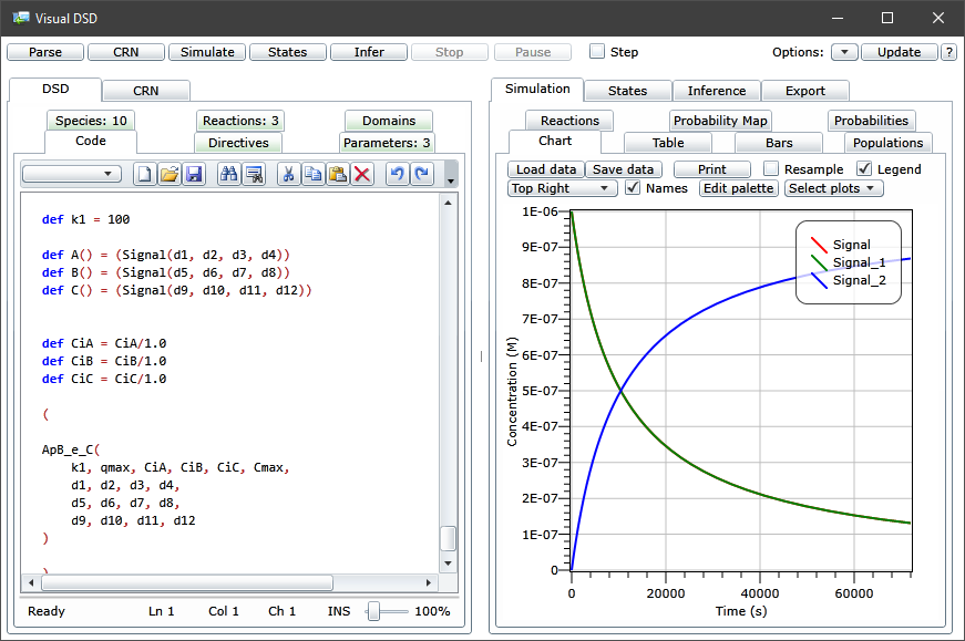
R session. Opening it with the Visual DSD and pressing "Simulate" in the top
left should leave you with a interface like this:
Note that we didn't specified a DNA-based CRN nor a device with the Visual DSD language in any step. We've made from a formal CRN to a DSD-based device directly without any particular knowledge of the specification language used by Visual DSD nor the approach used to translate a formal CRN do a DNA-based one.
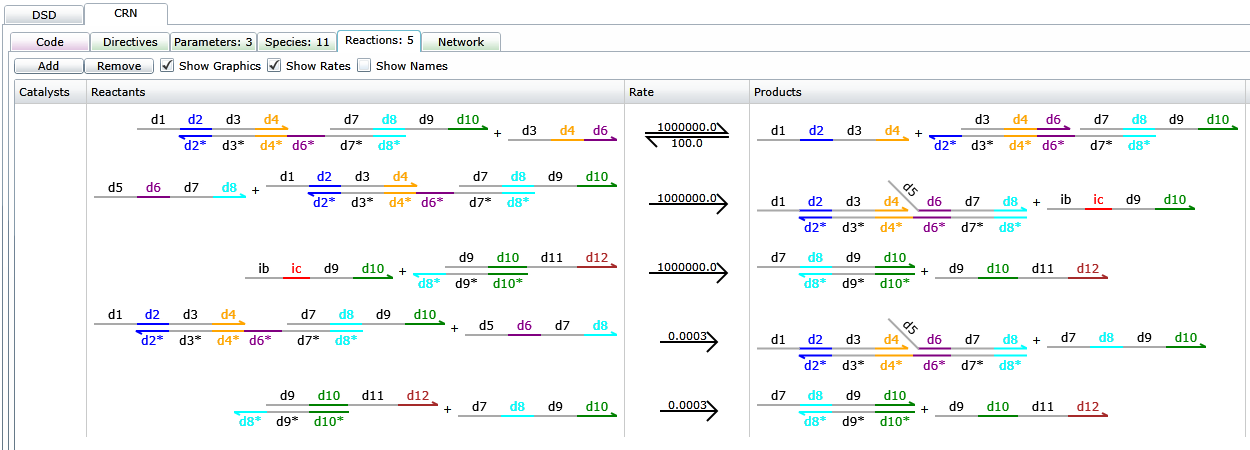
And finally, you can use Visual DSD features to better understand the device's behavior. A cool example the next image, where you can see what reactions are actually happening, and even see how the domains are interacting with each other.
However, as mentioned before, the file generated should be used as a framework. In fact, this entire process is not intended to happen automatically. The user must have the knowledge to set realistic values for the parameters in the formal to DNA-based translation step, as well as understand the features available in the Visual DSD in order to enable more detailed analysis and react properly to the different responses of the software. The main point is to show how it easy it is to get started with the process.
The version of Visual DSD used in this simulation was v0.14-20160312-35147
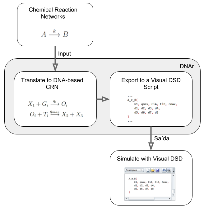
So, the image below summarizes the process described above.
One of the key features of DNAr that worths mentioning is its expandability.
Since DNAr provides its simulation capabilities through an API (and not
human-dependent interfaces), code can be written on top of DNAr to generate and
simulate large-scale complex CRNs. Furthermore, given the fact that the
implementations of react() and react_4domain() are independent, other
approaches of translating formal CRN into DNA-based ones can be implemented
without any change in the existent code (assuming that the approach also
yield a CRN as the of the translation).
A good example of this expandability can be shown using the approach of building neural networks discussed by [6].
The work of [6] presents an approach to implement a McCulloch–Pitts artificial neuron model (which is a binary neuron) using CRNs. Thus, the authors could build artificial neural networks and logic gates on top of that.
How the approach works is beyond the scope of this documentation, but we'll show how you can use an external implementation code to simulate logic gates designed with chemical artificial neurons, without even fully understanding how it works.
Within the DNAr package (R/neuron_hjelmfelt.R file), a set of functions
(which works as a plug-in for DNAr) were implement to build artificial chemical
neurons, artificial neural networks and some logic gates (AND, OR, Majority
gate). For this documentation, we'll stick to the most basic example: the
stand-alone neuron.
To define a neuron, we do the following:
n <- get_neuron_hje('n0', input_ci = 0.9)With this, we have defined a neuron with input 0.9. The activation rule for this neuron
is:
- activated: if the input concentration is
<= 0.9; - deactivated: if the input concentrations is
>= 1.1.
Between 0.9 and 1.1, the neuron's behavior gets undefined.
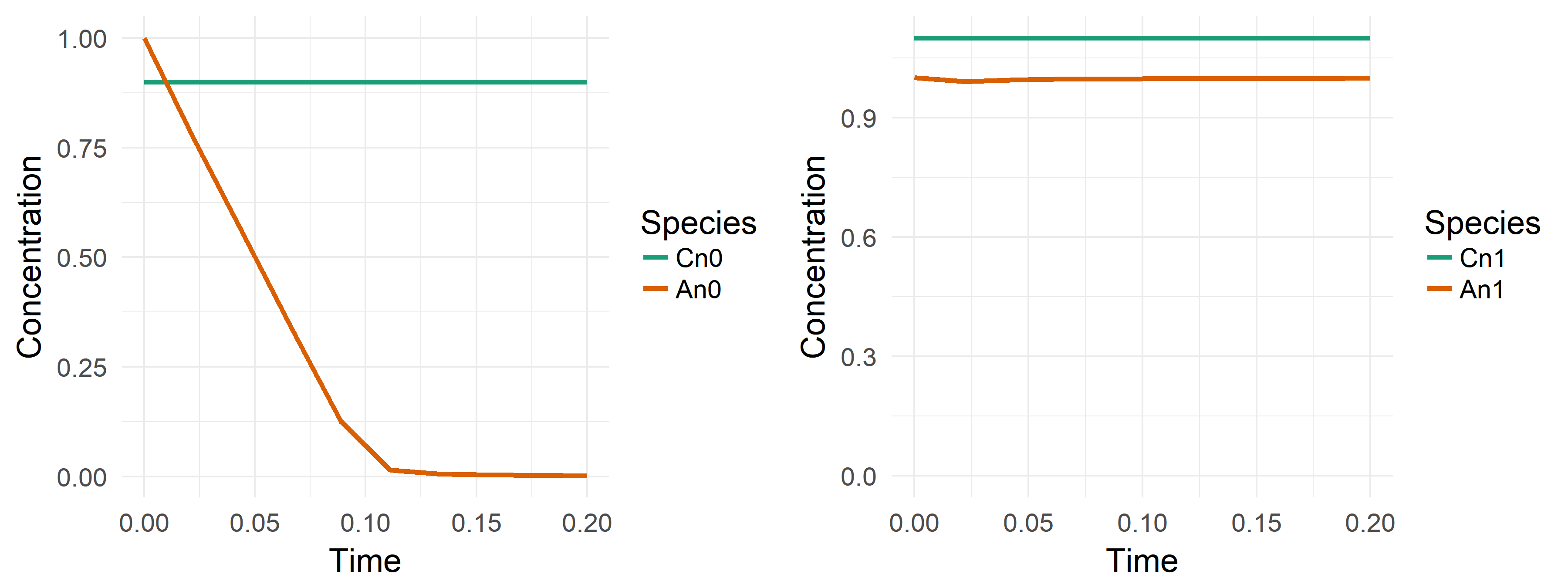
So, all the CRN is defined in n, therefore we can simulate it and see the
behavior of the species which defines its behavior:
Cn0: the input species;An0: defines the neuron state. If it's different than 0, the neuron is activated.
b <- react(
    species   = n$species,
    ci        = n$ci,
    reactions = n$reactions,
    ki        = n$ki,
    t         = seq(0, 0.2, length.out = 10)
)

plot_behavior(b, species = c('Cn0', 'An0'))
The result of the above simulation is the left side of the below Figure. The
right side is the result when input_ci = 1.1.
And if you want to simulate a DNA-based CRN of the neuron, it is also fairly
direct to do it. The only concern is to define proper values for qmax and
cmax. For the purpose of this documentation, values direct dependent of
the neuron CRN parameters are defined. alpha and beta are used just to
rescale the other CRN parameters (see [1]), therefore we'll leave them equal
1 to keep the other parameters as they are.
r <- react_4domain(
    species   = n$species,
    ci        = n$ci,
    reactions = n$reactions,
    ki        = n$ki,
    t         = seq(0, 0.2, length.out = 10),
    cmax      = max(n$ci) * 1e4,
    qmax      = max(n$ki) * 1e4,
    alpha     = 1, beta = 1
)

plot_behavior(r$behavior, species = c('Cn0', 'An0'))
Other good plug-ins implemented as separated packages are:
- DNAr-Logic [8] : Contains a set of functions implementing the approach of [7] of building logic gates directly with CRNs.
- DNAr-Analog [9] : Contains a set of functions implementing many analog computing gates directly with CRNs.
These plug-ins implemented as separated packages serves as good examples on how other pieces of software can be built on top of DNAr to create and simulate much more complex CRNs, focusing less on the Chemical Kinetics theory particularities, and more in higher level abstractions in order to solve problems.
The rule of thumb is this: If the code can yield a formal CRN with all the
parameters required by react(), it can be built on top of DNAr. So feel free
to implement a plug-in yourself. Two good yet not done examples of approaches
to build CRNs for a specific purposes are [2] and [3].
-
[1] Soloveichik, David, Georg Seelig, and Erik Winfree. "DNA as a universal substrate for chemical kinetics." Proceedings of the National Academy of Sciences 107.12 (2010): 5393-5398.
-
[2] Napp, N. E. & Adams, R. P. (2013). Message passing inference with chemical reaction networks. Em Advances in neural information processing systems, pp. 2247--2255.
-
[3] Zechner, C. & Khammash, M. (2016). A molecular implementation of the least mean squares estimator. Em Decision and Control (CDC), 2016 IEEE 55th Conference on, pp. 5869--5874. IEEE.
-
[4] Chen, Y.-J.; Groves, B.; Muscat, R. A. & Seelig, G. (2015). Dna nanotechnology from the test tube to the cell. Nature nanotechnology, 10(9):748--760.
-
[5] Lakin, M. R.; Youssef, S.; Polo, F.; Emmott, S. & Phillips, A. (2011). Visual dsd: a design and analysis tool for dna strand displacement systems. Bioinformatics, 27(22):3211--3213.
-
[6] Hjelmfelt, A.; Weinberger, E. D. & Ross, J. (1991). Chemical implementation of neural networks and turing machines. Proceedings of the National Academy of Sciences, 88(24):10983--10987.
-
[7] Jiang, H.; Riedel, M. D. & Parhi, K. K. (2013). Digital logic with molecular reactions. Em Computer-Aided Design (ICCAD), 2013 IEEE/ACM International Conference on, pp. 721--727. IEEE.
-
[8] Marks, R. A.; Vieira, D. K. S.; Guterres, M. V.; Oliveira, P. A. C. & Neto, O. P. V. (2019). DNAr-logic: a constructive DNA logic circuit design library in R language for molecular computing. In Proceedings of the 32nd Symposium on Integrated Circuits and Systems Design (SBCCI '19). Association for Computing Machinery, New York, NY, USA, Article 12, 1–6. DOI:https://doi.org/10.1145/3338852.3339854
-
[9] Oliveira, P. A. C.; Marks, R. A.; Teixeira, J. V. C.; Guterres, M. V.; & Neto, O. P. V. (2022). DNAr-analog: a library with a multiplexer to easily design, program, and simulate DSD analog circuits. (To appear): In Proceedings of the International symposium and flagship event of the IEEE Circuits and Systems Society in Latin America (LASCAS 2023).
