To get started with running the code in this repository you need to install the dependencies listed in
requirements.txt. Doing this is simply a matter of running the following command:
pip install -r requirements.txt
The above command should be enough to get code working. However, it is also recommended you use a conda environment. Install conda from:
https://docs.anaconda.com/anaconda/install/
Then open a terminal and run:
conda create --name breakstrat
conda activate breakstrat
conda install pip
pip install -r requirements.txt
Make sure that your project interpreted points to the conda environment (e.g. breakstrat) you have created for this repository.
Description
The baseline strategy is based on a simple heuristic for identifying a breakout. The heuristic boils down to looking at recent prices over a fixed time window, and comparing those prices to the current price. The current price level is classified as a breakout if the direction of change is positive and also significantly different from the price movements observed in the recent past (in our chosen time window).
There are two definitions for "significantly different" that we experiment with:
- ABS: Looks at the maximum absolute value of return over the given time window. If the last return divided by the maximum absolute value of return exceeds a predetermined threshold, then the current price level is considered a breakout.
- SDEV: Looks at the standard deviation of log return over the given time window. If the last log return is a given number of standard deviations larger then the current price level is considered a breakout.
For a more precice definition of the above look at the is_breakout function in the strategies/common.py module.
Once a breakout is detected a trade is entered. A trade is entered using a buy limit order. The limit order is placed one period in advance, at the minimum level price needs to reach in the next period in order to be considered a breakout.
There are three possible ways in which a trade is exited. We can either hit our stop loss or target level. In the case that neither levels are hit we exit after a fixed number of time has passed since we entered. The baseline sets a stop loss at a fixed percentage below the price the trade was entered at. Similarly, the take profit is set at a fixed percentage above the entry price.
Example backtest command:
python -m strategies.baseline.backtest
    --data_path=data/binance_spot_eth_usdt_1min.json
    --breakout_method=sdev
    --alpha=0.5
    --beta=2.0
    --stop_coeff_initial=0.985
    --target_coeff=1.15
    --terminal_num_periods=20
    --lookback=60
lb_breakoutdetermines how sensitive the breakout detection algorithm is. Higher values forlb_breakoutrequire the difference between the current price vs. past prices to be more significant.stop_coeff_initialis the fraction to multiply the entry price by to get the stop loss level.target_coeffis the fraction that determines the level at which to take profit. The level is based on the price that a trade is entered at.terminal_num_periodsis the maximum number of periods that a position is held for. If neither the target level nor the stop level is hit a trade is exited when the terminal number of periods is reached.lookbackis used by the breakout detection algorithm. It determines the number of past periods required to establish whether a breakout has occurred.
The output of a backtest is saved in the directory specified by --run_dir (default runs/trailstop_[timestamp]).
Results
The backtest period from 2020-03-01T06:00:00Z until 2020-08-20T20:12:00Z. In order for a strategy to be profitable (after fees) the average return per trade needs to exceed 1.002. Our baseline strategy was able to achieve profitability on the 5min data for both ETHUSDT and BTCUSDT. On the 1min data the baseline strategy failed to attain profitability. Performance on ETHUSDT was better than on BTCUSDT.
ABS
| data_path | cum_return | avg_return_per_trade | num_trades | num_pos_trades | num_neg_trades |
|---|---|---|---|---|---|
| data/binance_spot_eth_usdt_1min.json | 9.4123 | 1.00127 | 1801 | 631 | 1170 |
| data/binance_spot_eth_usdt_5min.json | 3.50452 | 1.00362 | 357 | 161 | 196 |
| data/binance_spot_btc_usdt_1min.json | 4.30364 | 1.00086 | 1746 | 495 | 1251 |
| data/binance_spot_btc_usdt_5min.json | 2.64223 | 1.0028 | 359 | 164 | 195 |
python -m strategies.baseline.backtest --data_path=data/binance_spot_eth_usdt_1min.json --breakout_method=abs --lb_breakout=1.0 --stop_coeff_initial=0.985 --target_coeff=1.15 --terminal_num_periods=20 --lookback=60
python -m strategies.baseline.backtest --data_path=data/binance_spot_eth_usdt_5min.json --breakout_method=abs --lb_breakout=1.0 --stop_coeff_initial=0.985 --target_coeff=1.15 --terminal_num_periods=20 --lookback=60
python -m strategies.baseline.backtest --data_path=data/binance_spot_btc_usdt_1min.json --breakout_method=abs --lb_breakout=1.0 --stop_coeff_initial=0.985 --target_coeff=1.15 --terminal_num_periods=20 --lookback=60
python -m strategies.baseline.backtest --data_path=data/binance_spot_btc_usdt_5min.json --breakout_method=abs --lb_breakout=1.0 --stop_coeff_initial=0.985 --target_coeff=1.15 --terminal_num_periods=20 --lookback=60
SDEV
| data_path | cum_return | avg_return_per_trade | num_trades | num_pos_trades | num_neg_trades |
|---|---|---|---|---|---|
| data/binance_spot_eth_usdt_1min.json | 7.56887 | 1.00117 | 1773 | 620 | 1153 |
| data/binance_spot_eth_usdt_5min.json | 3.42524 | 1.0036 | 353 | 160 | 193 |
| data/binance_spot_btc_usdt_1min.json | 3.73697 | 1.00077 | 1743 | 494 | 1249 |
| data/binance_spot_btc_usdt_5min.json | 2.67037 | 1.00288 | 353 | 162 | 191 |
python -m strategies.baseline.backtest --data_path=data/binance_spot_eth_usdt_1min.json --breakout_method=sdev --alpha=0.5 --beta=2.0 --lb_breakout=1.0 --stop_coeff_initial=0.985 --target_coeff=1.15 --terminal_num_periods=20 --lookback=60
python -m strategies.baseline.backtest --data_path=data/binance_spot_eth_usdt_5min.json --breakout_method=sdev --alpha=0.5 --beta=2.0 --lb_breakout=1.0 --stop_coeff_initial=0.985 --target_coeff=1.15 --terminal_num_periods=20 --lookback=60
python -m strategies.baseline.backtest --data_path=data/binance_spot_btc_usdt_1min.json --breakout_method=sdev --alpha=0.5 --beta=2.0 --lb_breakout=1.0 --stop_coeff_initial=0.985 --target_coeff=1.15 --terminal_num_periods=20 --lookback=60
python -m strategies.baseline.backtest --data_path=data/binance_spot_btc_usdt_5min.json --breakout_method=sdev --alpha=0.5 --beta=2.0 --lb_breakout=1.0 --stop_coeff_initial=0.985 --target_coeff=1.15 --terminal_num_periods=20 --lookback=60
Figure 1
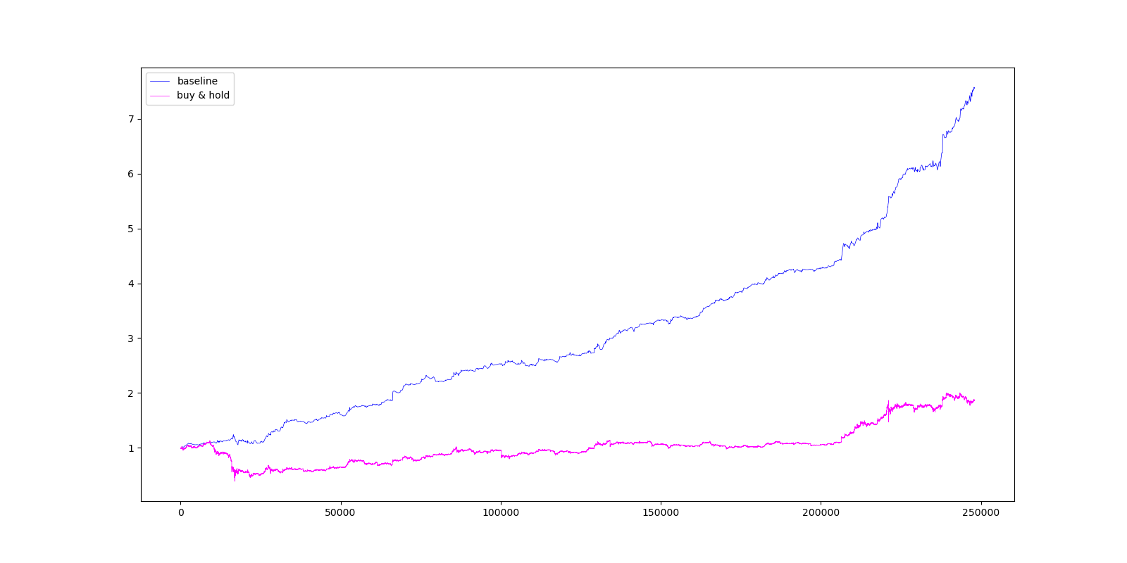
The output of a backtest contains a plot of the cumulative return of a strategy compared to buy and hold. Figure 1 shows the plot that is produced when running:
python -m strategies.baseline.backtest --data_path=data/binance_spot_eth_usdt_1min.json --breakout_method=sdev --alpha=0.5 --beta=2.0 --lb_breakout=1.0 --stop_coeff_initial=0.985 --target_coeff=1.15 --terminal_num_periods=20 --lookback=60
Figure 2
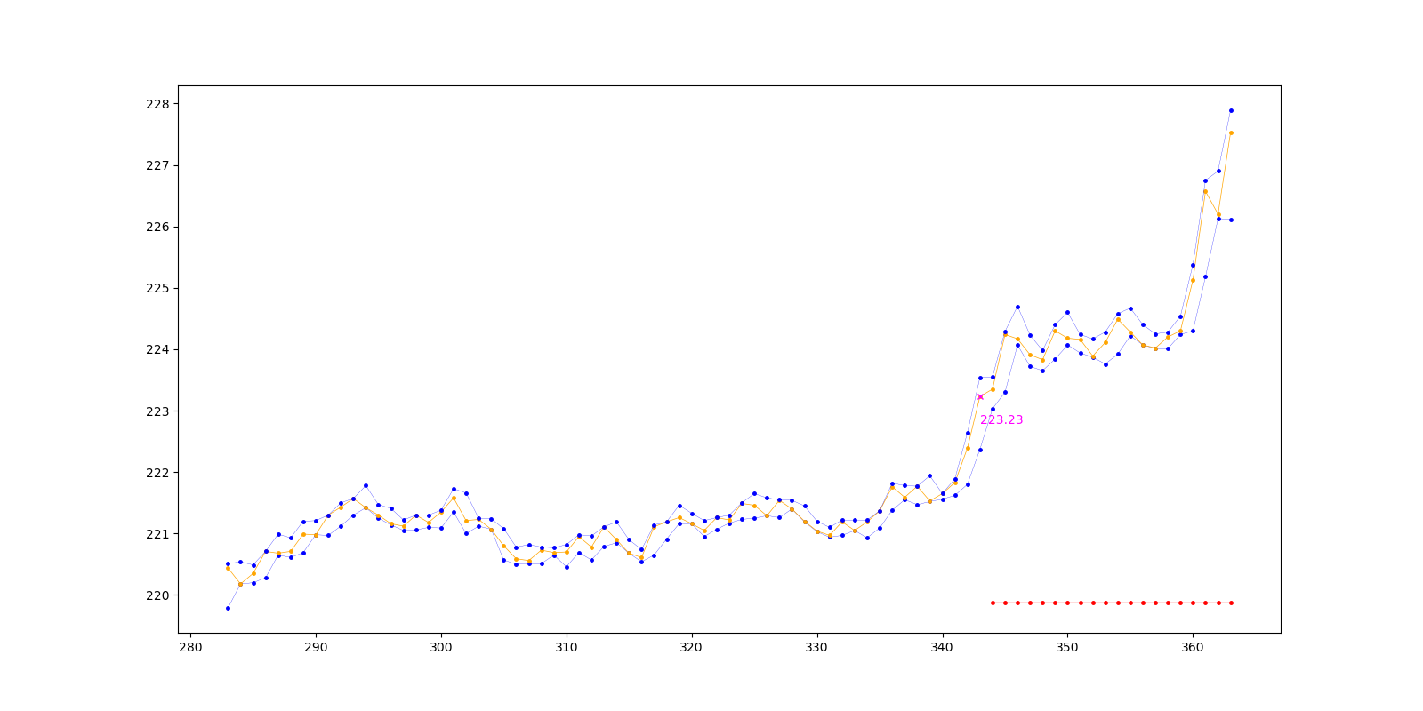
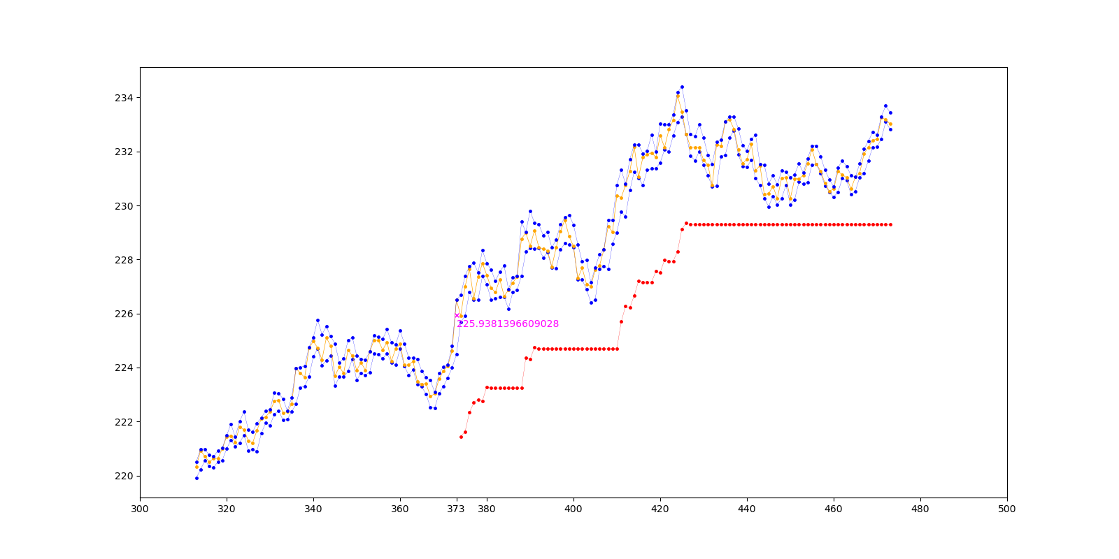
This is an example of a trade made by the baseline algorithm. The red line is the stop loss level. The number in
magenta is the price the algorithm entered the trade at. To produce this plot run the strategies/baseline/backtest.py
module but with --with_plots flag included. E.g.
python -m strategies.baseline.backtest
    --with_plots
    --data_path=data/binance_spot_eth_usdt_5min.json
    --lb=1.0
    --stop_coeff_initial=0.985
    --target_coeff=1.15
    --terminal_num_periods=20
    --lookback=60
Description
Trailstop is an extension of the baseline breakout strategy. The baseline strategy places a stop loss at a fixed level below the price at which a trade is entered. Trailstop instead uses a trailing stop loss based on a fixed percentage below the most recent high.
Results
E.g. command used to produce backtest results:
python -m strategies.trailstop.backtest
    --data_path=data/binance_spot_eth_usdt_5min.json
    --stop_coeff_initial=0.985
    --stop_coeff=0.99
    --target_coeff=1.15
    --terminal_num_periods=20
    --lookback=60
stop_coeff_initialis the fraction that determines the stop loss of the first period (after entry).stop_coeffis the fraction that determines the stop loss of subsequent periods. We found that setting an initial stop loss that is slightly lower performed better.- All other parameters are the same as the baseline strategy.
Table 1
| data_path | cum_return | avg_return_per_trade | num_trades | num_pos_trades | num_neg_trades |
|---|---|---|---|---|---|
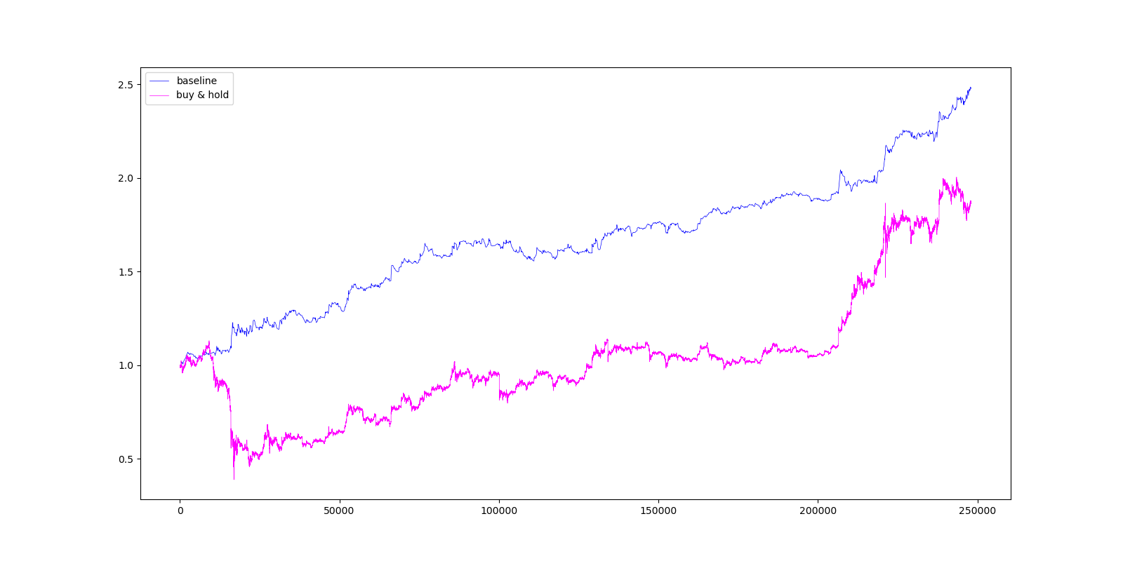
| data/binance_spot_eth_usdt_1min.json | 2.48227 | 1.00052 | 1817 | 889 | 928 |
| data/binance_spot_eth_usdt_5min.json | 2.38982 | 1.00245 | 363 | 175 | 188 |
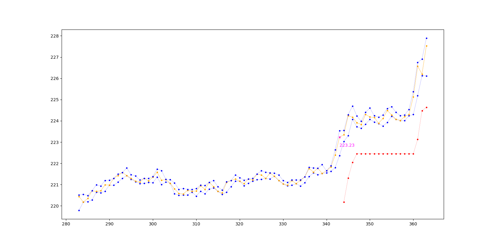
This is an example of a trade that was made by the trailstop algorithm. The red line is the stop loss level. Like the
baseline strategy, in order to produce this plot make sure to run the backtest module with --with_plots included.
Results
The command to run a backtest is:
python -m strategies.oustop.backtest
Table 1: ETHUSDT 5min
| data_path | cum_return | avg_return_per_trade | num_trades | num_pos_trades | num_neg_trades |
|---|---|---|---|---|---|
| data/binance_spot_eth_usdt_5min.json | 3.87865 | 1.00522 | 280 | 115 | 165 |
To reproduce run the backtest command with the following parameters:
{
    "lb_breakout": 1.005,
    "alpha": 0.5,
    "beta": 2.0,
    "target_coeff": 4.6,
    "terminal_num_periods": 100,
    "lookback": 60,
    "est_method": "max_abs_diff",
    "est_sigma_lag": 100,
    "theta": 2.0,
    "pred_method": "start_at_peak",
    "breakout_method": "abs",
    "data_path": "data/binance_spot_eth_usdt_5min.json"
}
Figure 1
The above figure shows an example of a successful trade made by OUstop.
Table 2: BTCUSDT 5min
| data_path | cum_return | avg_return_per_trade | num_trades | num_pos_trades | num_neg_trades |
|---|---|---|---|---|---|
| data/binance_spot_btc_usdt_5min.json | 2.22937 | 1.00311 | 292 | 109 | 183 |
The parameters used to produce the above table are the same as with ETHUSDT 5min. The only difference is the data_path
parameter.
| data_path | cum_return | avg_return_per_trade | num_trades | num_pos_trades | num_neg_trades |
|---|---|---|---|---|---|
| data/binance_spot_eth_usdt_5min.json | 4.36392 | 1.00411 | 367 | 148 | 219 |
| run_dir | data_path | num_trades | num_pos_trades | num_neg_trades | prob_true |
|---|---|---|---|---|---|
| runs/trailstop_1599403704228716 | data/binance_spot_eth_usdt_5min.json | 357 | 172 | 185 | 0.481793 |
| runs/trailstop_1599480765138089 | data/binance_spot_eth_usdt_1min.json | 1747 | 854 | 893 | 0.488838 |
The above table is saved in research/results/baseline.md. To produce this table run the following command:
python -m research.baseline --run_ids "[1599403704228716, 1599480765138089]"
Remarks:
- The estimate of the probability of a true breakout is biased. The estimate rests on the assumption that a true breakout corresponds to a profitable trade (defined by Trailstop). However, there are a lot of examples of profitable trades that intuitively we wouldn't want to classify as being true breakouts (see figure *). Despite this issue, the current working definition does still provide a rough idea of the probability of a true breakout. More importantly, the definition is likely good enough to test whether certain features are predictive for a true breakout.
In this section we investigate whether volume correlates with the probability of a breakout. I.e. are certain values of volume more likely to correspond to a true breakout than others? The belief that we test is that a breakout on larger volume is more likely to be a true breakout.
The results below are generating using the python -m research.volume command.
Table 1
| lb | volume_interval | prob_true | num_obs |
|---|---|---|---|
| 1 | [33.46566, 321.89743] | 0.478022 | 182 |
| 1 | [4603.93268, 31713.3321] | 0.508287 | 181 |
| 1.0025 | [33.46566, 335.12007] | 0.141243 | 177 |
| 1.0025 | [4703.96199, 31713.3321] | 0.357955 | 176 |
| 1.005 | [33.46566, 335.43794] | 0.0285714 | 175 |
| 1.005 | [4790.58909, 31713.3321] | 0.241379 | 174 |
| 1.01 | [33.46566, 335.43794] | 0.0115607 | 173 |
| 1.01 | [4798.95866, 31713.3321] | 0.127907 | 172 |
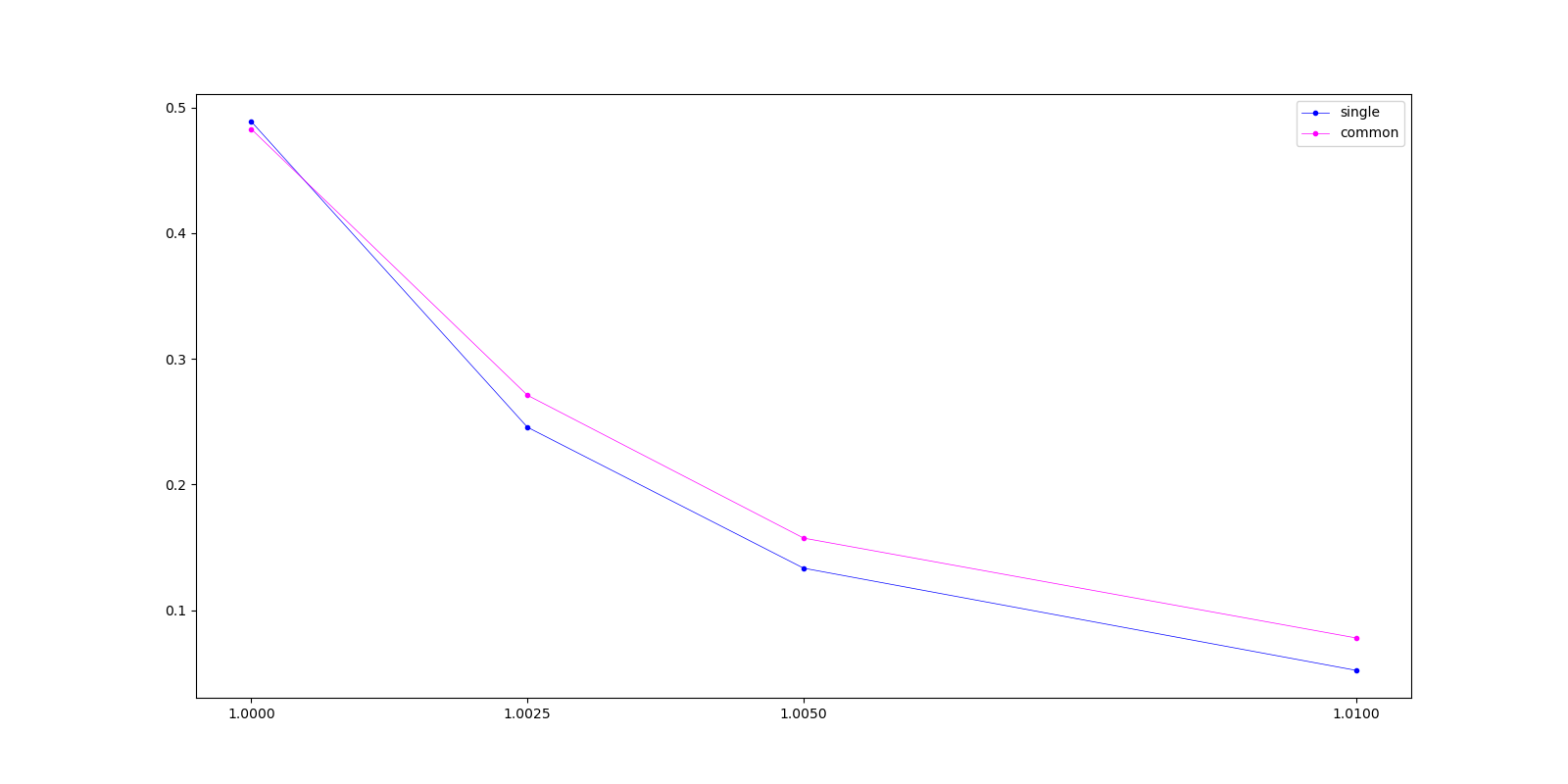
The above table looks at the probability of a true breakout at different levels of volume. E.g. the first row shows the (estimated) probability of a true breakout when the volume (at the time of breakout) is between is between 33.56566 and 335.43794. The num_obs column displays the number of observations that went into estimating the probability.
This figure shows the same information as the above table. The values on the x-axis correspond to the row numbers of the table; the y-axis to the probability of a true breakout.
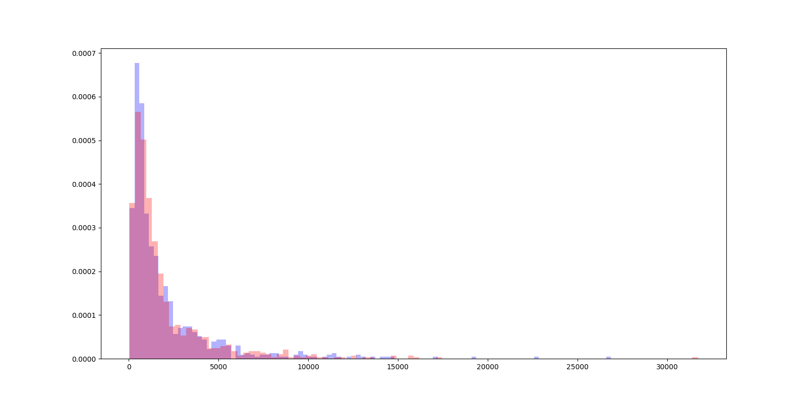
The above figure is a histogram of the volume at breakout time for all trades. The red histogram corresponds to breakouts that were false (i.e. unprofitable). The blue histogram corresponds to true breakouts.
The results on data/binance_spot_eth_usdt_5min are similar. To view those results simply go into the
research/results/volume_eth_usdt_5min directory.
| lb | prob_true | prob_true_common | num_true_signals | num_signals | num_true_common_signals | num_common_signals |
|---|---|---|---|---|---|---|
| 1 | 0.130985 | 0.150685 | 238 | 1817 | 99 | 657 |
| 1.0025 | 0.133144 | 0.155624 | 235 | 1765 | 101 | 649 |
| 1.005 | 0.133371 | 0.157321 | 233 | 1747 | 101 | 642 |
| 1.01 | 0.13476 | 0.157566 | 233 | 1729 | 101 | 641 |
In this section we are interested in answering the questions: Is it possible to predict a true breakout using past returns? If we had a large enough dataset i.e. were most possible returns series preceding a breakout are observed (multiple times), then answering this question is relatively straightforward. To estimate the conditional (on past returns) probability of a true breakout, one could simply use a nearest neighbor approach. The density (of data) in a neighborhood would be sufficient to get a reliable estimate.
Besides the neareset neighbor approach, there are numerous other conditional probability models that can be used to obtain an estimate. Regerdless of the method used, the reliability of our estimate relies heavily on the density of the data surrounding the corresponding returns series.
There are two main factors that affect the density of data: (1) The dimensionality of our returns series, and (2) the amount of data we have. In this section we will focus on the first issue: dimensionality. In particular, we will focus on finding alternative lower dimensional representations (i.e. embeddings) of returns. The aim is to create embeddings that are a good enough summary of the orginal returns series, whilst having a much lower dimensionality, therefore signficantly improving the density of our data.
The first approach we try out maps any series into a 2-dimensional representation. The rule is extremely simple. We just look at the mean and standard deviation of the returns that make up a returns series. The mean and standard deviation are sufficient statistics for estimating the parameters of a Geometric Brownian Motion (GBM). The GBM is a stochastic process that is a simple (but commonly used) model for financial time series (see https://en.wikipedia.org/wiki/Geometric_Brownian_motion).
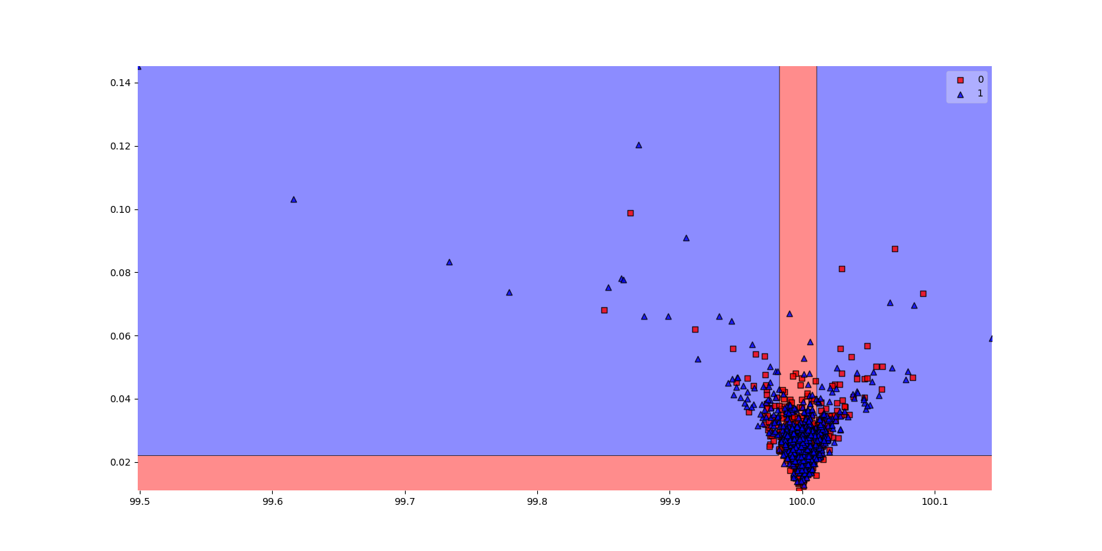
Using the above idea we convert all return sequences to 2-dimensional feature vectors. We then use a decision tree to segment this feature space into regions of different probability of (true) breakout. Before fitting the decision tree the data is down-sampled to make the number of false breakouts equal to the number of true breakouts in the data. (The number of false breakouts overwhelms the number of true breakouts. Without down-sampling the decision tree is unable to segment the feature space. Every point in the feature space ends up being classified as a false breakout.)
Results
The results below are produced by running:
python -m research.embed
    --symbol=binance_spot_eth_usdt_1min
    --embedder_type=gbm
    --max_depth=4
    --min_samples_leaf=60
    --lb_return=1.002
Figure 1
The segmentation of the feature space learned by the decision tree (on down-sampled data). Blue dots correspond to true breakouts; red dots to false breakouts. The blue regions correspond to areas where the probability of a true breakout is higher than average.
Table 1
| group | prob_pos | num_pos | num_obs | avg_return_per_trade |
|---|---|---|---|---|
| 11 | 0.358804 | 324 | 903 | 1.00115 |
| 13 | 0.48951 | 70 | 143 | 1.00224 |
| 7 | 0.5 | 66 | 132 | 1.00372 |
| 14 | 0.382716 | 31 | 81 | 1.0026 |
| 10 | 0.430233 | 37 | 86 | 1.00201 |
| 3 | 0.203704 | 22 | 108 | 1.00033 |
| 5 | 0.336066 | 41 | 122 | 1.00128 |
| 4 | 0.168605 | 29 | 172 | 1.00009 |
The decision tree segements the feature space into multiple regions (or groups). In the above table group 13 and 7 are notable. The reason is that the average return of a trade in those regions is larger than 1.002; as such, are profitable in the long run.
Table 2
| prob_true_given_pred_pos | prob_neg_given_pred_neg | prob_pos | prob_neg | num_obs | num_pos | num_neg | num_pred_pos | num_pred_neg | num_true_pos_and_pred_pos | num_true_neg_and_pred_neg |
|---|---|---|---|---|---|---|---|---|---|---|
| 0.461538 | 0.681226 | 0.354894 | 0.645106 | 1747 | 620 | 1127 | 442 | 1305 | 204 | 889 |
This table shows the probability of a breakout conditional on the predictions made by the decision tree (used to segment the feature space). E.g. If the decision tree predicts a returns series corresponds to a true breakout, there is a 46.1% chance that this is indeed the case.
Caveat(s):
- The results are for the training data. Performance on unseen data is yet to be determined.
- The number of observations in each group is small; arguably not enough to be confident.
Our GBM method can be a bit crude in representing a return series. The problem, especially for longer series, is that the underlying process that generates returns tends to change after a certain period of time. In this case, using a single GBM may not be expressive enough. To remedy this issue we try out a simple extension. We split our returns series into two pieces (down the middle). We then calculate the mean and standard deviation of each piece seperately. The mean and standard deviation of each piece are then combined (into a single vector) to create a 4-dimensional representation of the original return series.
Note: The decision to split the returns series down the middle is a crude heuristic. Ideally, the point to split at should be at a change point. (For a definition and examples of the term change point see https://tinyurl.com/yxrp2n7k). Implementing a change point detection algorithm is a possible future extension of GBMSplit.
Results
| group | prob_pos | num_pos | num_obs | avg_return_per_trade |
|---|---|---|---|---|
| 17 | 0.361878 | 262 | 724 | 1.00097 |
| 20 | 0.551402 | 59 | 107 | 1.00372 |
| 19 | 0.403846 | 42 | 104 | 1.00147 |
| 13 | 0.594595 | 44 | 74 | 1.00655 |
| 10 | 0.308176 | 49 | 159 | 1.00091 |
| 11 | 0.214286 | 18 | 84 | 1.00018 |
| 4 | 0.227273 | 20 | 88 | 1.00027 |
| 8 | 0.396552 | 46 | 116 | 1.0017 |
| 16 | 0.442105 | 42 | 95 | 1.00205 |
| 6 | 0.284211 | 27 | 95 | 1.00116 |
| 5 | 0.108911 | 11 | 101 | 1.00013 |
| prob_true_given_pred_pos | prob_neg_given_pred_neg | prob_pos | prob_neg | num_obs | num_pos | num_neg | num_pred_pos | num_pred_neg | num_true_pos_and_pred_pos | num_true_neg_and_pred_neg |
|---|---|---|---|---|---|---|---|---|---|---|
| 0.405738 | 0.762808 | 0.354894 | 0.645106 | 1747 | 620 | 1127 | 1220 | 527 | 495 | 402 |
