Implementation of our MICCAI and invited IJCARS paper on detecting anatomical landmarks of the pelvis in X-ray images from arbitrary views.
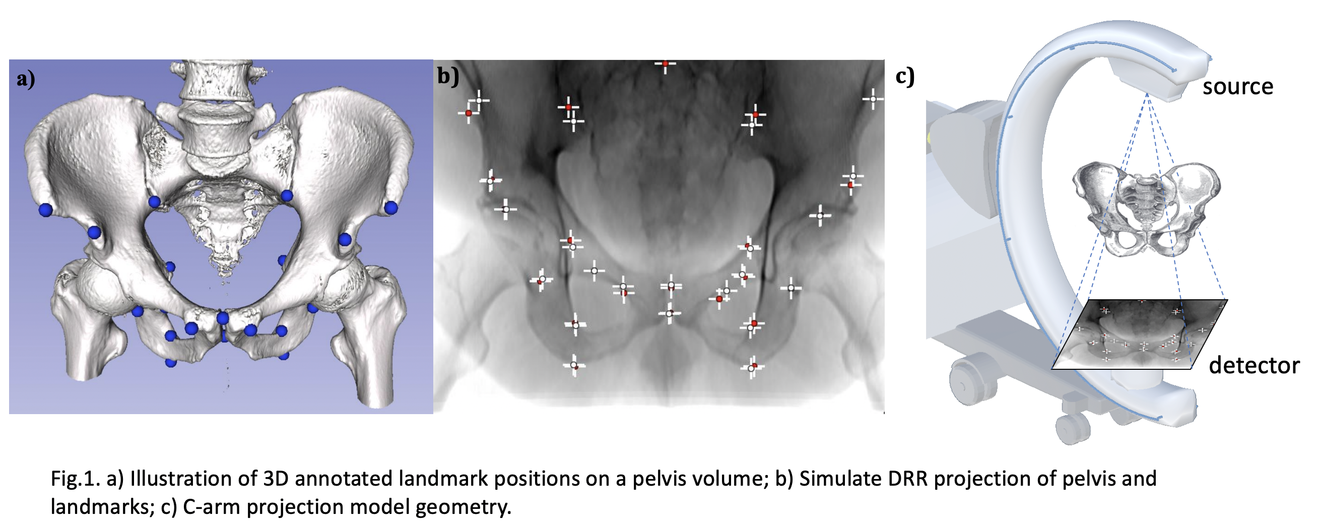
Our training data is synthetically generated from full body CTs from the NIH Cancer Imaging Archive [1]. In total, 20 CTs (male and female patients) were cropped to an ROI around the pelvis and 23 anatomical landmark positions were annotated manually in 3D. Landmarks were selected to be clinically meaningful and clearly identifiable in 3D; see Fig. 1 a). We release our annotation files under the folder './annotation/Labels'. The name of the .fcsv file is in consistent with the CT data. We also release the CT origin offset under the folder './annotation/origin.txt'
Dicom Offset: The CT volume offset is recorded in the dicom meta data. The dicom slices need to be sorted according to the tag (0020, 0013). Then the dicom offset can be read from tag (0020,0032) in the first slice after sorting.
Origin Offset: We calibrated the CT volume in our C-arm geometry by adding an origin offset. The calibrated origin data is uploaded in the text file 'origin.txt'.
The 3D annotation landmark point is noted as landmark3D. The aforementioned dicom offset is noted as dicom_offset; origin offset as origin_offset. Please use the following sudo code to manipulate the landmark offset.
landmark3D[0] = -(landmark3D[0] + dicom_offset[0]) + origin_offset[0]
landmark3D[1] = -(landmark3D[1] + dicom_offset[1]) + origin_offset[1]
landmark3D[2] =   landmark3D[2] - dicom_offset[2]  + origin_offset[2] - 25
After this, we can then use the conventional pinhole camera projection model to project the 3D landmark onto 2D plane. We note the 3-by-4 projection matrix as P. The 3-by-1 projected result is saved at proj. The 2D landmark coordinate is saved at landmark2D.
proj = P * [landmark3D; 1] # Make it homogeneous coordinate
landmark2D[0] = proj[0] / proj[2]
landmark2D[1] = proj[1] / proj[2]
We provide a matlab code projection.m with numeric examples to better undrestand the above process. The code takes the CT file: ABD_LYMPH_057 as an example, where the dicom offset and origin are
 DICOM offset Tag (0020, 0032): [-199.61, -380.83, -686.80]
 Instance number Tag (0020, 0013): 1
 Origin Offset: [-206, -224, -118]
We use the first annotated landmark position: [30.45, 122.19, -630.07], and generate a random rotation and translation matrix saved as R and T. The 3-by-3 C-arm intrinsic calibration matrix is saved as K.
During our pipeline training, we resized the heatmap prediction dimension for memory concern. The original simulated image dimension is 479-by-615 with pixel size 0.616mm. We then downsampled it to 59-by-76 as network output. During evaluation, we loaded the network prediction result and upsampled back to the original resolution to compare with the groundtruth position.
In order to understand our evaluation process, we provide an example code, which uses a single pelvis image prediction heatmaps (23 landmarks * 6 stages = 138 imgs) and its corresponding 2D groundtruth positions to calculate the l2 distance loss. The files and python code can be found in the floder './evaluation'.
[1] Roth, H., Lu, L., Seff, A., Cherry, K.M., Hoffman, J., Wang, S., Summers, R.M.: A new 2.5 d representation for lymph node detection in ct. The Cancer Imaging Archive (2015)