This repo contains the information and pipeline used to analyze data for wholebrain cFos mapping.
This document is useful to have a self-contained explanation of the pipeline used to analyze the cFos for the Monogenic (MG) project. Hopefully it works to help keep organized the many files/stages involved in this experiment.
We will be working with a tree structure that looks like this
.
├── MG847
├── MG884
├── MG886
├── MG889
├── MG927
├── MG952
└── ...
Briefly:
raw_datawill have animal folders by name (“MG[0-9]+”).- Each animal folder will contain the
.czifiles and a number of folders created by the pipeline.c0->> DAPI (registration channel)c1->> cFOS (segmentation channel)c2->> if neededcompositeswill have the.tiffcomposites (2 or 3 channels).
Files are named with this general pattern
Below, I detail the pipeline, describing what will be done by each of the R scripts used to run it.
Images come from the scanning microscope in .czi format. They might
have 2 or 3 channels (DAPI and cFos is the standard).
They should be kept in a folder named by the corresponding animal_id
(see folder structure).
The script batch_czi_to_tiff.ijm will ask for folder where .czi
images are stored. It takes quite a while to export all images.
CAUTION: For some reason, images are repeated. You will find the same image at many resolutions. Sort by name, and only choose the ones with high size (>500 MB).
Create a folder named 001 and move all big .tif files there.
Now, you can continue with the pipeline.
First, it will rename files (removing some extra tags that the
batch_czi_to_tiff.ijm script adds). Second, it will call a python
script named batch_composite_to_single_tiff.py to separate files into
proper channels, creating proper folders to contain them (i.e., c0,
c1, …).
This step takes between 5 and 10 minutes and a progress bar will show the processing.
The call to python currently uses this python.
“/home/mike/miniconda3/bin/python”
It might fail when executed from another computer. To check where is your python located, run from command line:
which python
Adjust python commands properly.
This script is the bulk of processing, with several steps of manual processing.
Choose the folder of the animal you are working with.
We need to resize our images (make them smaller, add padding). This
takes some minutes per animal and it will print progress to console. The
base function is resize_pad.R. It will save output into a folder
called small.
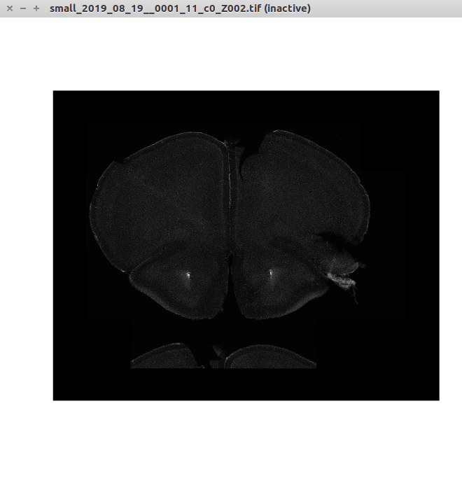
From the small images, we can read and find the biggest contour using
find_contours.R. We will use these contours to pass to the
registration functions.
The following command will prompt the user to match the images to Atlas
# image folder being the place where the small DAPI images are
image_folder <- file.path(root_path, "small")
match_df <- match_image_to_atlas(image_folder)
It will display the original small image and an equalized one (know shown).
It will prompt the user with:
what is your first guess for AP level? :>
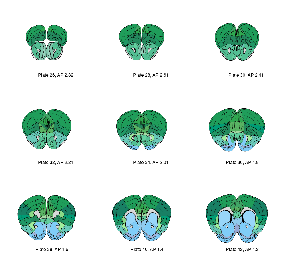
And call pull_atlas around that AP level (example shown for AP = 2).
It will prompt user with options:
+++++++++++++++++++++++++
Please see your options below:
+++++++++++++++++++++++++
Option 1) 2.82
Option 2) 2.61
Option 3) 2.41
Option 4) 2.21
Option 5) 2.01
Option 6) 1.8
Option 7) 1.6
Option 8) 1.4
Option 9) 1.2

Use numbers to select the option that best fits your image :>
And loop for decision making.
The result is an object of class data.frame with 2 columns:
names(match_df)
[1] "image_file"     "mm.from.bregma"
We could have matched 2 images to the same AP level. Moreover, we could
have made a mistake during the assignment. Thus, we use the function
inspect_AP_match to check for duplicates and make sure all assignments
were correct.
This function will show you the image and the pull_atlas(AP) for the
AP you selected during the previous matching. It will prompt you to
solve incorrect assignments and duplicates.
Now we are ready to rename our images with a Z number that indicates
the order from anterior to posterior. This is needed for the SMART
pipeline to work.
CAUTION: We chose not to duplicate files to save space. Thus, once you rename with a Z plane, the files will no longer be able to be read by the previous steps that rely on the original file path.
The function call is
match_df_2 <- rename_AP(match_df_2)We get a new data.frame, similar to the previous one, and files get
renamed properly.
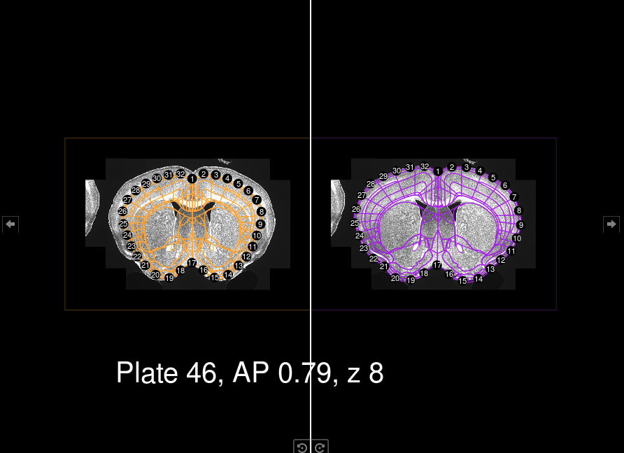
SMART is built around a setup object that gets created with
setup_pl() and modified by a family of functions. We can by-pass that
by direct assignment of values (For this case, it’s easier this way).
We know reorder the lists of contours and matched images so that they are fed in the proper order to the pipeline.
This is done using regi_loop and it takes a while. It might make
errors, so we have to later inspect the images. There is a helper
function that we can call by doing:
plates <- inspect_wrong_regi_plates(setup)This will show the registration files living in the folder
registration_auto and registration_manual (if you happen to already
done some manual registration)
It will prompt the user to define whether they want to perform manual
registration on that image or not. At the end of the loop, the object
plates will hold all the plates that need to be registered manually.
Thus, the following call will perform manual fix of selected plates:
# Manual fix of registration ####
regi_loop(setup, regis = regis,
          touchup = plates, brightness = 20,
          filter = ordered_filter_list, autoloop = FALSE)
Changes will be saved onto the regis object created by regi_loop.
Now we have all contours. We need to extract them from the regis
object and select those of our interest. We use prep_data function and
a series of subsetting/renaming calls to perform these steps.
We also match them with the EPSatlas.RData coming from wholebrain.
This data.frame contains all the naming conventions that we need to be
able to get our regions of interest.
The fundamental part is selecting the correct acronyms. Below, there’s an example for 5 “parent” regions. We will get all the “children” for them and use them to filter our contour list.
# We need to translate from acronym to structure_id
# We have to choose the parents of the structures we care about and use a recursive get children
# This comes from SMART package
rois <- get_all_children(c("ILA", "PL", "BLA", "MOp", "SSp"))
Finally, all contours of interest will be saved as data.frames in a
folder called contours. This will be done as 1 .csv file per image.
Now that we have the contours of interest we can prepare the python call
to make the croppings. Croppings are made by a series of functions
inside read_large.py. They will read the original size images (stored
in c0, c1, …), rescale the regions of interest to the original size and
perform cropping.
The croppings will be moved by an R function called move_crops. This
call will be inside a for loop of each channel
for(i in 1:length(c0_files)){
  # make the call by pasting arguments c0
  # system(...)
  # move_crops()

  # make the call by pasting arguments c1
  # system(...)
  # move_crops()

}
This is quite verbose, so the user should be able to follow. Progress will be printed.
To make sure the contours are properly rescaled, it might be good to call this function with
-display_contours Trueat least in c0 channel. This is currently not working perfectly from command line (all contours/crops will be displayed) and it will slow down computation.
We get all the images and group them by region. Because the partition is
not reproducible (involving sample_frac()), we save the partition list
to be able to later follow what happened (i.e., what image went where).
We can put all the images back by reversing the rename.files() call to
move files back from the training/testing folder to the composites
folder.
We are now ready to move to iLastik to perform pixel classification assisted by human labeling.


