How can a machine learning model be trained to classify flowers? The fundamental question behind this is how a machine learning model categorizes data like the flower pictures. Adaline (Adaptive Linear Neuron) is a good example for machine learning classification.
How is this related to gradient descent? Adaline starts with a random decision boundary, and computes the cost function of it. Then gradient descent can be used to minimize the cost function and move the decision boundary to its optimized location.
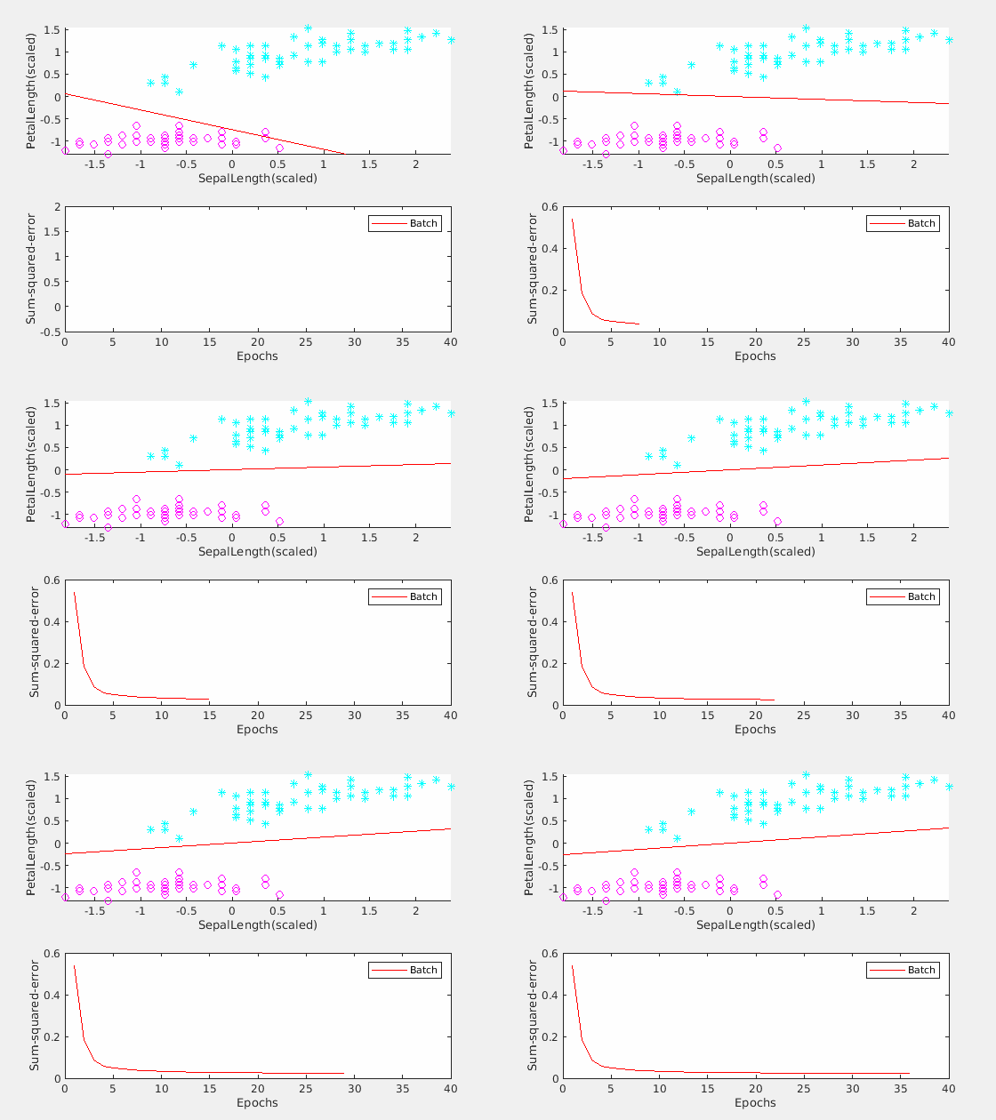
Note if a picture is worth a thousand words, an animation shall worth more than a thousand pictures. Animated Adaline is a MATLAB® class that visualizes how an Adaline model is trained. More specifically, Animated Adaline can show how each iteration of gradient descent lowers down the cost function, thus moves the decision boundary at the same time. For beginners, this demonstrates clearly how gradient descent is used to do machine learning classification.
Please refresh the browser to restart the animation.
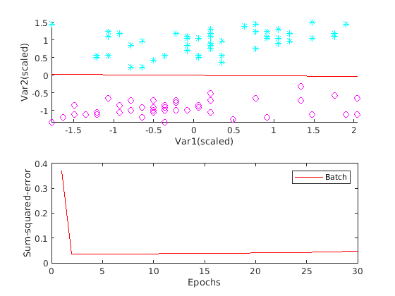
In the above animation, the top one is a scatter plot of some data from the iris dataset from UCI server. The red line is the decision boundary. The lower one is a plot of the cost function of an Adaline model.
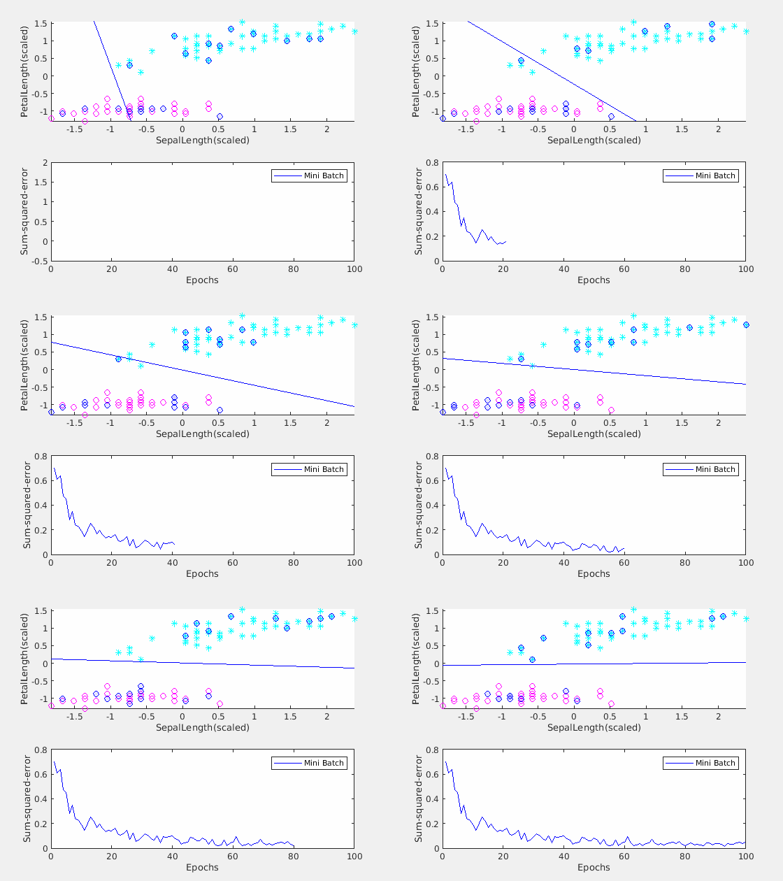
In addition to normal (batch) gradient descent, Animated Adaline also supports mini batch and stochastic gradient descents. For advanced deep learning users, it can be used to demonstrate the related concepts. Animated Adaline highlights the subgroup of data being used to do mini batch for each iteration of gradient descent. Users can see clearly how this subgroup affects the moving of the decision boundary.
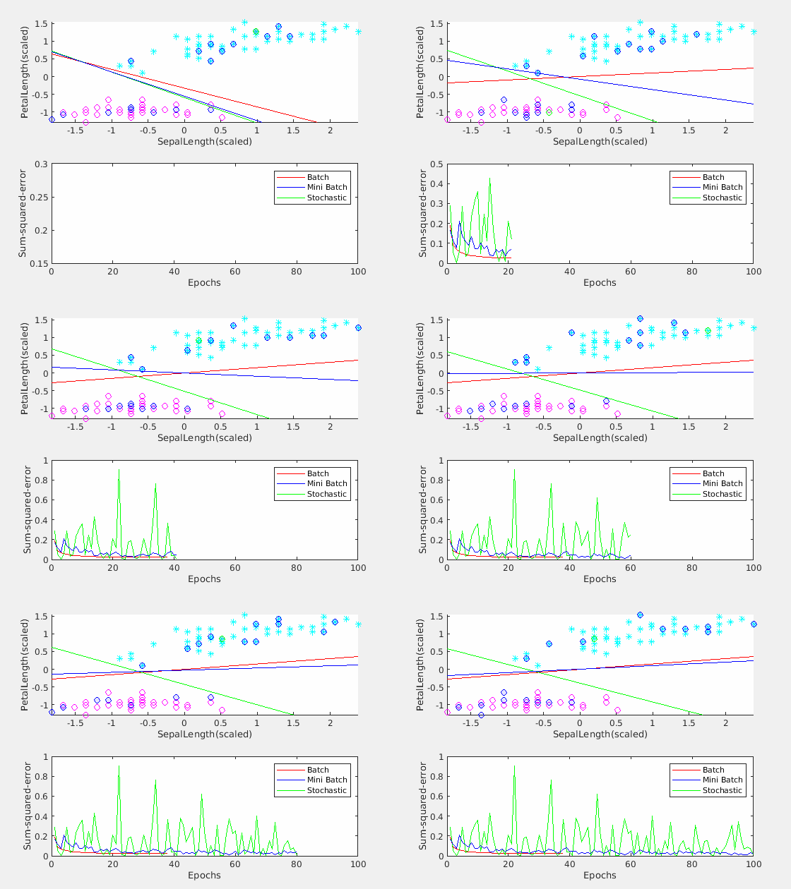
Users can even compare these three different kinds of gradient descent by animating them at the same time.
Features:
- Support batch, mini batch, and stochastic gradient descent. Plot them independently or all together
- Plot decision boundary and cost function for each iteration of gradient descent
- Allow user to set learning rate alpha to demonstrate its impact
- Allow user to set mini batch size to see how it affects the training process
- Allow user to use his/her own data set
- Generate animation gif for a presentation or course materials
See test.m for simple examples for getting started quickly.
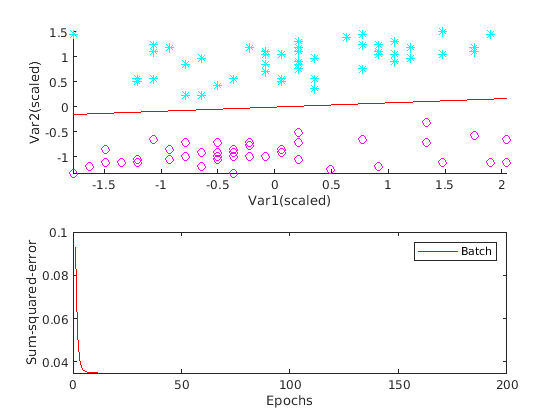
Instantiate it with the data file. Note this uses a bogus dataset included with this script.
ada = Adaline('sample_data.csv');
If you just want to use default settings, then you can start the animation (See Example 1 in test.m)
ada.animate();
As shown above, the bogus dataset contains two categories/classes (plotted in cyan and in magenta in the top scatter plot). The red line in the top plot is the decision boundary. When the training is finished, the decision boundary successfully separates the two classes.
By default, only batch gradient descent is turned on. You can use the following three member variables to turn on/off them individually. The following example shows the mini batch only.
ada = Adaline('sample_data.csv');
ada.showBatch = false;          % skip batch gradient descent
ada.showMiniBatch = true;       % show minibatch
ada.showStochastic = false;     % skip stochastic
ada.maxSteps = 100;             % maximum iterations of gradient descent
ada.showHighLight = true;       % high light min batch samples
ada.animate();
The above example also show how to to stop the gradient descent by setting the maximum iteractions of gradient descent.
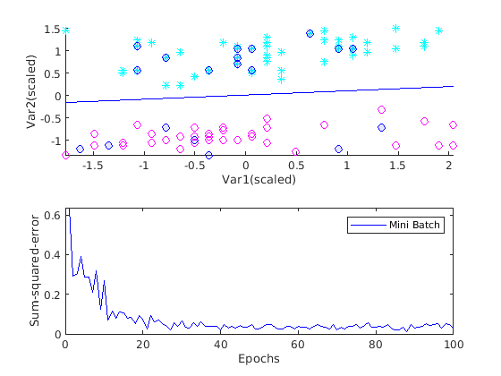
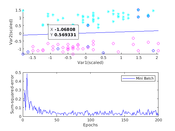
The cost function plot is not as smooth as the one of the batch gradient descend, because the optimized solution for a subgroup (the mini batch) of samples is in general not the same as the optimized solution for the whole group. By setting the showHighLight property, the subgroup of samples are highlighted as shown in the above screenshot of the animation.
If you set all three gradient descents to be true, you can then generate an animation similar to the third one from top of this page.
Set the learning rate (before calling animate).
ada.alpha = 0.0155; % a big learning rate
This learning rate is closed to the threshold. Bigger alpha will make the cost function diverge. Visually the decision boundary moves away from the opimized location.
Set mini batch size by doing this
ada.batchSize = 10; % smaller batch size
By default, mini batch size is 20. By setting a smaller size, the cost function plot oscillates more than the Mini Batch plot above, which uses the default size of 20.
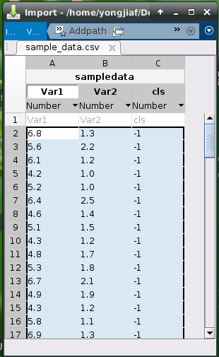
A bogus dataset is included for illustration purpose. It is saved in CSV format.
A script is provided to download and process the iris dataset from UCI server.
The dataset you provided needs to be three columns. The first one is the first feature, the second one is the second feature. The third one needs to be the label. It must be either 1 or -1. If you want to use your own dataset, save it into a format like the bogus data, then it can be used by Animated Adaline.

