Once completing pre-processing in eeglab/erplab/Net Station, you’re
ready to get to the fun stuff: plotting and measuring with EPP-TB! This
package is aimed at simple (readable), concise (one function per action)
and reproducible code writing. Additionally, a major component is the
ability to export data and plots to be used and further manipulated
elsewhere (say, ggplot2?).
All user-end functions start with epp_*.
To use EPP-TB you will need:
- Matlab (2015a+).
- eeglab (14.X.X) for
importing
.setfiles, and plotting topos. - R (for plotting in R)
You can install the package by downloading and adding the EPP-TB folder (and sub-folders) to your Matlab paths.
Three import methods are currently supported:
epp_loadeeglab- Import multiple.setfiles from eeglab (supports wavelet analysis based on Mike X. Cohen’s great book and code).epp_loaderplab- Import from erplab.epp_loadegimat- Import multiple.matfiles exported from Net Station (EGI).
The resulting structure array has length(struct) equal to the number
of conditions, and contains the following fields, per condition:
- Condition: the name of the conditions.
- timeLine: a vector of time points.
- IDs: a table with two variables - ID and nTrials (the number of trials a ERP has been averaged across).
- Data: a
channelsxtime pointsxSubjectsmatrix for ERP data.
If a wavelet analysis has been preformed, the Data field is replaced with:
-
ersp and itc:
channelsxfrequenciesxtime pointsxSubjectsmatrices. -
Freqs: a vector of frequencies used.
These functions can be used to compute new conditions or manipulate existing data:
- Merge 2 or more conditions with
epp_combineconds(). - Compute differences between 2 conditions with
epp_diffwave(). - Compute LRP with
epp_LRP() - Compute global field potentials with
epp_GFP(). - Collapse TF data to frequency waveforms with
epp_reshapeTF(). - Make grand-average ERP/ERSP/ITC with
epp_makegrands()(useful for plotting large data sets).
- Add data to
study.IDsfrom a table withepp_appendID(). - Retain subjects that have data in all specified conditions with
epp_matchsubjects(). - Select data from specific subjects by some variable in
study.IDswithepp_filter_by(). - Pull data from
study.IDswithepp_extractIDs().
For all
epp_plot*functions, which allow plotting data fromeppstructures, there is an accompanying generalp_*function, that allows plotting from other data structures (with a little bit of wrangling).
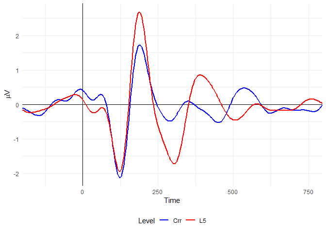
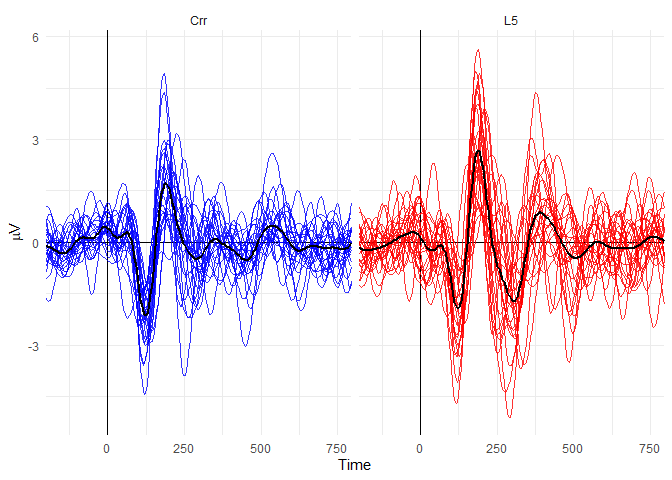
Grand averages can be plotted by specifying the conditions and channel indices (averaged across) to plot:
conds         = {'Crr','L5'};
channel_inds  = [5 6 11 12];
epp_plotgrands(study,conds,channel_inds)
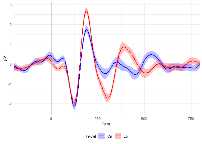
You can also plot error envelopes:
epp_plotgrands(study,conds,channel_inds,'errorType','SE')
% can also be set to 'SD' or 'CIXX'
% (with XX replaced with any percent: 'CI95','CI80', etc...).
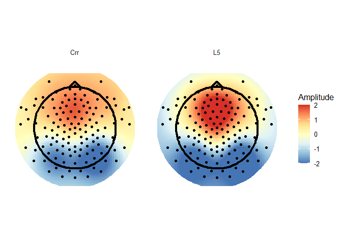
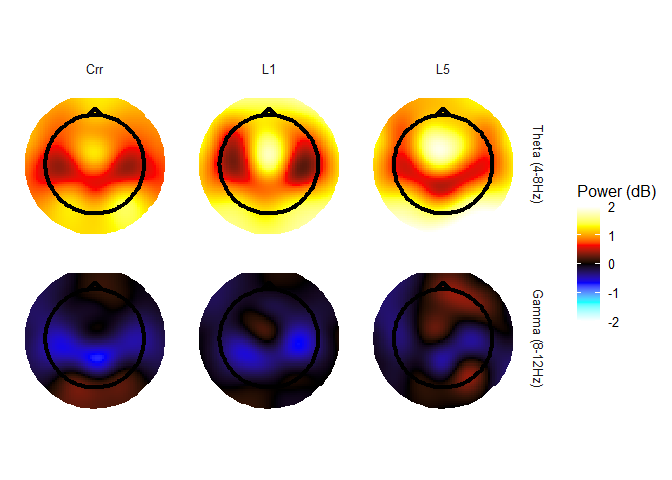
Topo plotting is dependent on eeglab functions. Additionally, you will
need to provide a eeglab-like chanlocs structure to these functions,
with length(chanlocs)==size(study.Data,1).
times = [185];
epp_plottopo(study,chanlocs,conds,channel_inds,times)
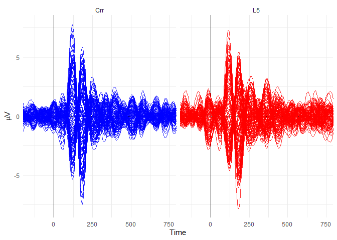
Butterfly plots can be used to plot the mean ERP for each subject individually.
epp_plotbutterfly(study,conds,channel_inds)Trace plots are similar to butterfly plots, but the mean activation (across subjects) is plotted for each channel separately.
channel_inds = []; % if left blank, all channels are plotted.
epp_plotbutterfly(study,conds,channel_inds,'trace',true)Similar to trace plots, channel plots give a picture of what is
happening at each channel (like eeglab’s plottopo). These come in
two flavors:
- Topo Plots - channel data is plotted in 2-d space, like a topo-plot.
- Grid Plots - channel data is plotted on a simple grid.
Channel topo plots are created with the following Matlab call:
channel_inds = []; % if left blank, all channels are plotted.
epp_plotchannels(study,conds,electrodes,'chanlocs',chanlocs)
Grid plots are called using the same call, without providing chanlocs.
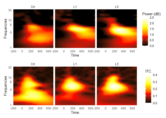
Time Frequency plots plot both ersp and itc:
epp_plotTF(study,conds,channel_inds)All the listed above plotting methods also support TF data. For example:
times = [160 410];
bands = [4 8; 8 12];
% a matrix of frequencies, with each row containing a range of frequencies
% to plot (1st column is lower limit, 2nd column is upper limit of band).
epp_plottopo(study,chanlocs,conds,channel_inds,times,...
'freqs',bands, 'type', 'ersp')All plots can be exported to R and plotted with
ggplot2 by setting 'R',true
in any of the plotting function (this is how the plots in this README
were made). This produces two time-stamped files:
- A data file (
*_data.csv) - A code file (
*_code.R), to plot said data usingggplot2.
Measuring can be done via the epp_get* functions. These are wrapper
functions for the various m_* functions (with one functions per
method), which should not be called directly (unless you know what
you’re doing).
Saving results always produces a 2-sheet .xlsx file, with the second
sheet containing the parameters used in measuring - this is to insure
reproducibility of results. Thus, if you have the output .xlsx file,
you’ll never find yourself asking “what was the time window we used last
time?”.
The function epp_getAmp implements the methods for measuring
amplitudes described in chapter 9 of Steven J. Luck’s intro to ERP
book.
- (Local) Peak amplitude
- Point amplitude
- Mean amplitude
- Integral
- Area
The function epp_getLat implements the methods for measuring latencies
described in chapter 9 of Steven J. Luck’s intro to ERP
book,
as well as those described in Kiesel et al.’s Jakknife
paper.
- (Local) Peak latency
- Relative criterion
- Fractional area
- Baseline deviation
- Absolute criterion
The function epp_getTF measure the mean ersp / itc from selected
channels, within a specified time-window,separately for specified
frequency bands (as shown above, for epp_plottopoTF).
- Mattan S. Ben-Shachar [aut, cre].
- Rachel Rac [ctb].
- Michael Shmueli [ctb].
- Mike X. Cohen - who’s
code was implemented in
f_WaveletConv.m. - Matt Craddock - who’s
code was
implemented in
epp_plottopo.R. - Winston Chang - who’s
code
for computing within-subject (and mixed model) CI’s was implemented
in
epp_plotgrands.m.
