This package literally consists of one function - a method for
converting lavaan objects into tbl_graph objects.
This function has been copied to MSBMisc and will be maintained there.
You can install tidylavaan from
github with:
# install.packages("devtools")
devtools::install_github("mattansb/tidylavaan")

# or just load the single function it contains:
# source("https://raw.githubusercontent.com/mattansb/tidylavaan/master/R/tidylavaan.R")
These functions are meant for use alongside
tidygraph and
ggraph (as seen bellow).
You will also need:
- lavaan, obviously.
In this example we will try to recreate the plot in the main page of
lavaan’s website:
Let’s first fit the model:
library(lavaan)## Warning: package 'lavaan' was built under R version 3.6.1
model <- '
   # latent variables
     ind60 =~ x1 + x2 + x3
     dem60 =~ y1 + y2 + y3 + y4
     dem65 =~ y5 + y6 + y7 + y8
   # regressions
     dem60 ~ ind60
     dem65 ~ ind60 + dem60
   # residual covariances
     y1 ~~ y5
     y2 ~~ y4 + y6
     y3 ~~ y7
     y4 ~~ y8
     y6 ~~ y8
'
fit <- sem(model, data = PoliticalDemocracy)Using tidylavaan we can convert this object into a tbl_graph object:
library(tidygraph)
library(tidylavaan)

graph_data <- as_tbl_graph(fit, standardize = TRUE)
Wow, that was super hard. Let’s see what we got.
print(graph_data)## # A tbl_graph: 14 nodes and 20 edges
## #
## # A directed acyclic simple graph with 1 component
## #
## # Node Data: 14 x 2 (active)
## name latent
## <chr> <lgl>
## 1 ind60 TRUE
## 2 dem60 TRUE
## 3 dem65 TRUE
## 4 y5 FALSE
## 5 y4 FALSE
## 6 y6 FALSE
## # ... with 8 more rows
## #
## # Edge Data: 20 x 11
## from to op est.std se z pvalue ci.lower ci.upper
## <int> <int> <chr> <dbl> <dbl> <dbl> <dbl> <dbl> <dbl>
## 1 1 9 =~ 0.920 0.0230 40.0 0 0.875 0.965
## 2 1 10 =~ 0.973 0.0165 59.1 0 0.941 1.01
## 3 1 11 =~ 0.872 0.0311 28.1 0 0.811 0.933
## # ... with 17 more rows, and 2 more variables: relation_full <chr>,
## # relation_type <chr>
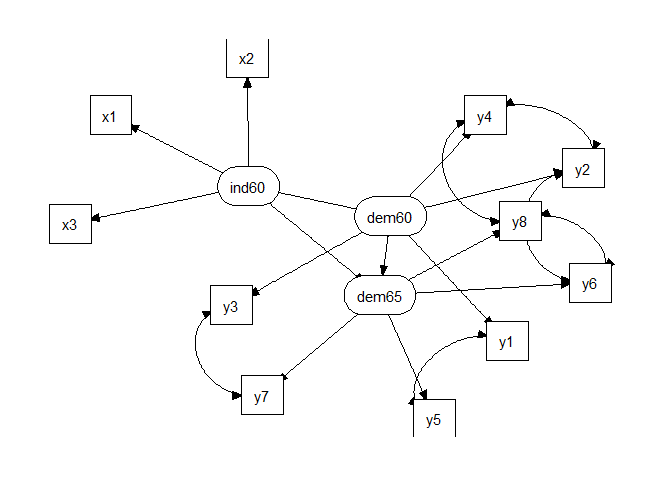
Let’s plot it with ggraph (learn more about plotting nodes and
edges).
library(ggraph)## Warning: package 'ggplot2' was built under R version 3.6.1
graph_layout <- create_layout(graph_data, layout = "kk")

arrow_cap     <- circle(5, 'mm')
label_dodge   <- unit(2.5, 'mm')
label.padding <- unit(0.7,"lines")

ggraph(graph_layout) +
  # edges
  geom_edge_link(aes(filter = relation_type == "regression"),
                 arrow     = arrow(20, unit(.3, "cm"), type = "closed"),
                 start_cap = arrow_cap,
                 end_cap   = arrow_cap) +
  geom_edge_arc(aes(filter = relation_type == "covariance"),
                arrow     = arrow(20, unit(.3, "cm"), type = "closed", ends = "both"),
                start_cap = arrow_cap,
                end_cap   = arrow_cap) +
  # nodes
  geom_node_label(aes(filter = !latent,
                      label  = name),
                  label.r       = unit(0, "lines"),
                  label.padding = label.padding) +
  geom_node_label(aes(filter = latent,
                      label  = name),
                  label.r       = unit(1.0, "lines"),
                  label.padding = label.padding) +
  # Scales and themes
  theme_graph()
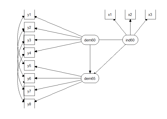
Not bad, but we can also specify the exact desired locations manually:
graph_layout$x <- c(3.5,2.5,2.5,1,1,1,1,1,3,3.5,4,1,1,1)
graph_layout$y <- -0.2*c(3,3,6,5,4,6,7,8,1,1,1,1,2,3)

ggraph(graph_layout) +
  # edges
  geom_edge_link(aes(filter = relation_type == "regression"),
                 arrow     = arrow(20, unit(.3, "cm"), type = "closed"),
                 start_cap = arrow_cap,
                 end_cap   = arrow_cap) +
  geom_edge_arc(aes(filter = relation_type == "covariance"),
                arrow     = arrow(20, unit(.3, "cm"), type = "closed", ends = "both"),
                start_cap = arrow_cap,
                end_cap   = arrow_cap) +
  # nodes
  geom_node_label(aes(filter = !latent,
                      label  = name),
                  label.r       = unit(0, "lines"),
                  label.padding = label.padding) +
  geom_node_label(aes(filter = latent,
                      label  = name),
                  label.r       = unit(1.0, "lines"),
                  label.padding = label.padding) +
  # Scales and themes
  theme_graph()
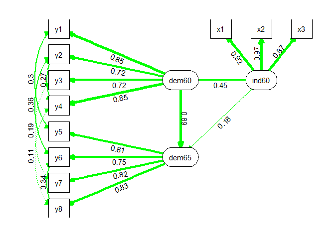
And now the world in our oyster! Let’s pretty it up!
ggraph(graph_layout) +
  # edges
  geom_edge_link(aes(filter   = relation_type == "regression",
                     width    = abs(est.std),
                     linetype = !pvalue < .05,
                     label    = round(est.std,2),
                     color    = est.std < 0),
                 angle_calc  = "along",
                 label_dodge = label_dodge,
                 arrow       = arrow(20, unit(.3, "cm"),type = "closed"),
                 start_cap   = arrow_cap,
                 end_cap     = arrow_cap) +
  geom_edge_arc(aes(filter   = relation_type == "covariance",
                    width    = abs(est.std),
                    linetype = !pvalue < .05,
                    label    = round(est.std,2),
                    color    = est.std < 0),
                angle_calc  = "along",
                label_dodge = label_dodge,
                arrow       = arrow(20, unit(.3, "cm"), type = "closed", ends = "both"),
                start_cap   = arrow_cap,
                end_cap     = arrow_cap) +
  # nodes
  geom_node_label(aes(filter = !latent,
                      label  = name),
                  label.r       = unit(0, "lines"),
                  label.padding = label.padding) +
  geom_node_label(aes(filter = latent,
                      label  = name),
                  label.r       = unit(1.0, "lines"),
                  label.padding = label.padding) +
  # Scales and themes
  scale_edge_color_manual(guide = FALSE, values = c("green","red")) +
  scale_edge_width_continuous(guide = FALSE, range = c(0.5,2)) +
  scale_edge_linetype_discrete(guide = FALSE) +
theme_graph()- Mattan S. Ben-Shachar [aut, cre].


