Presentation

This code performs some of the experiments in

O. Balabanov, M. Beaupere, L. Grigori, V. Lederer. Block subsampled randomized Hadamard transform for low-rank approximation on distributed architectures. View on arXiv.

Given a dense, large, distributed matrix $A$, we aim at computing a random sampling of $A$ (randomized, or sketched). It is further used to computing the Nyström low rank approximation of $A$.

Furthermore, it also serves the illustrations of my Ph.D thesis.

Conservation of the inner product through sketching.
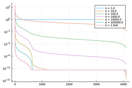
Obtain singular values from several datasets.

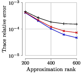
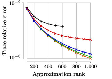
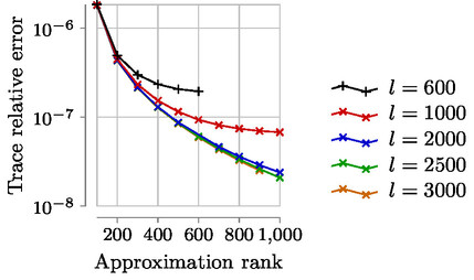
Instructions to reproduce the Nyström approximation experiments

Expected accuracy results (Datasets MNIST, Year with sigma=1000, Year with sigma=10 000):

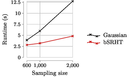
Expected runtime results:

Required software

The experiments were done under a Linux environment.

This program requires Julia version 1.7.2 with the following packages

TimerOutputs.jl
ClusterManager.jl
DistributedArrays.jl
Hadamard.jl.

Obtain the dataset

Download and extract the training and test datasets.

$> wget https://www.csie.ntu.edu.tw/\~cjlin/libsvmtools/datasets/multiclass/mnist.scale.bz2
$> wget https://www.csie.ntu.edu.tw/\~cjlin/libsvmtools/datasets/multiclass/mnist.scale.t.bz2
$> bzip2 -d mnist.scale.bz2
$> bzip2 -d mnist.scale.t.bz2

Concatenate datasets, merging 60 000 records from the training data and 5536 records from the testing data. The suffix specifying the feature count _780 is required for the program to work correctly.

$> cat mnist.scale > mnist_780
$> head -n 5536 mnist.scale.t >> mnist_780

Or build a datasets of 32 768 rows

$> head -n 32768 mnist.scale >> mnist_780

Execute the program

Load environment variables corresponding to the dataset.

$> source scripts/env/mnist.env

Start Julia

$> ./path/to/julia -p 64

And then start the script to reproduce the timings and the error.

julia> include("scripts/nystrom.jl")

The scripts in scripts/env can help to execute this on a cluster equipped with the Slurm scheduler.

Find the results

Timings

Look at the file timings_p64_kmin200_height65536.csv for the times in milliseconds. Columns are

The sampling parameter
The time of block SRHT
The time of TSQR
The time of SVD of R
The time of Gaussian sampling

Only (2) and (5) are given in the submitted paper.

Error

Look at the files nuclear_error_*.csv to get the relative trace error of each run.

Additional instructions

This section describes how to reproduces figures from my PhD thesis.

Nyström approximation of additional datasets

The previous step can be reproduced with other datasets:

Plot singular values for each dataset and different sigmas

Expected result for the MNIST dataset:

Use the scripts/plot_rbs_kernel_svd.jl file and modify the constants:

dataset_filename: Path to dataset.
sep: Dataset values separation character.
sigmas: Different values of sigma (see RBS kernel expression), each corresponding to a line in the plot.

Plot inner products conservation

Use the scripts/innerproducts.jl file. Call the main function with the wanted dataset (including random) and value for $l$, the sampling size.

matthiasbe/block_srht