ElastiK Nearest Neighbors

Insight Data Engineering Project, Boston, April - June 2018


Image similarity search demo running searches on a cluster of 4 Elasticsearch nodes

Overview

I built Elasticsearch-Aknn (EsAknn), an Elasticsearch plugin which implements approximate K-nearest-neighbors search for dense, floating-point vectors in Elasticsearch. This allows data engineers to avoid rebuilding an infrastructure for large-scale KNN and instead leverage Elasticsearch's proven distributed infrastructure.

To demonstrate the plugin, I used it to implement an image similarity search engine for a corpus of 6.7 million Twitter images. I transformed each image into a 1000-dimensional floating-point feature vector using a convolutional neural network. I used EsAknn to store the vectors and search for nearest neighbors on an Elasticsearch cluster.

The repository is structured:

demo directory: Twitter Image Similarity search pipeline and web-application
elasticsearch-aknn directory: EsAknn implementation and benchmarks
scratch directory: several smaller projects implemented while prototyping

Demo

~~Web-application~~ (Taken down at the end of the Insight program)
Screencast demo on Youtube
Presentation on Google Slides

Elasticsearch-Aknn

Usecase

EsAknn is useful for problems roughly characterized:

Have a large corpus of feature vectors with dimensionality ~50-1000.
Need to run similarity searches using K-Nearest-Neighbors.
Need to scale horizontally to support many concurrent similarity searches.
Need to support a growing corpus with near-real-time insertions. I.e., when a new vector is created/ingested, it should be available for searching in less than 10 minutes.

How does it compare to other approximate-nearest-neighbors libraries?

Tldr: If you need to quickly run KNN on an extremely large corpus in an offline job, use one of the libraries from Ann-Benchmarks. If you need KNN in an online setting with support for horizontally-scalable searching and indexing new vectors in near-real-time, consider EsAknn (especially if you already use Elasticsearch).

There are about a dozen high-quality open-source approximate-nearest-neighbors libraries. The Ann-Benchmarks project is a great place to compare them. Most of them take a large corpus of vectors, build an index, and expose an interface to run very fast nearest-neighbors search on that fixed corpus.

Unfortunately they offer very little infrastructure for deploying your nearest-neighbors search in an online setting. Specifically, you still have to consider:

Where do you store millions of vectors and the index?
How do you handle many concurrent searches?
How do you handle a growing corpus? See this issue on the lack of support for adding to an index.
How do you distribute the index and make searches fault tolerant?
Who manages all the infrastructure you've built for such a simple algorithm?

Elasticsearch already solves the non-trivial infrastrcture problems, and EsAknn implements approximate nearest-neighbors indexing and search atop this proven infrastructure.

EsAknn's LSH implementation is very simplistic in the grand scheme of approximate-nearest-neighbors approaches, but it maps well to Elasticsearch and still yields high recall. EsAknn's speed for serial queries is much slower than other approximate nearest-neighbor libraries, but it's also not designed for serial querying. Instead it's designed to serve many concurrent searches over a convenient HTTP endpoint, index new vectors in near-real-time, and scale horizontally with Elasticsearch. For specific performance numbers, see the performance section below and the slides linked in the demo section.

API

Create LSH Model

Given a sample of vectors, create a locality-sensitive-hashing (LSH) model and store it as an Elasticsearch document.

POST <elasticsearch host>:9200/_aknn_create 

{
    "_index":   "aknn_models",
    "_type":    "aknn_model",
    "_id":      "twitter_image_search",
    "_source": {
        "_aknn_description": "LSH model for Twitter image similarity search",
        "_aknn_nb_tables": 64,
        "_aknn_nb_bits_per_table": 18,
        "_aknn_nb_dimensions": 1000
    },
    "_aknn_vector_sample": [
        # Provide a sample of 2 * _aknn_nb_tables * _aknn_nb_bits_per_table vectors
        [0.11, 0.22, ...],
        [0.22, 0.33, ...],
        ...
        [0.88, 0.99, ...]
    ]
}

This returns:

{ "took": <number of milliseconds> }

Index New Vectors

Given a batch of new vectors, hash each vector using a pre-defined LSH model and store its raw and hashed values in an Elasticsearch document.

POST <elasticsearch host>:9200/_aknn_index

{
    "_index":       "twitter_images",
    "_type":        "twitter_image",
    "_aknn_uri":    "aknn_models/aknn_model/twitter_image_search"
    "_aknn_docs": [
        {
            "_id": 1,
            "_source": {
                "_aknn_vector": [0.12, 0.23, ...],

                # Any other fields you want...
            }
        }, ...
    ]
}

This returns:

{ "took": <number of milliseconds>, "size": <number of documents indexed> }

Similarity Search

Given a vector in the index, search for and return its nearest neighbors.

GET <elasticsearch host>:9200/twitter_images/twitter_image/1/_aknn_search?k1=1000&k2=10

This returns:

{
    "took": <number of milliseconds>,
    "timed_out": false,

    "hits": {
        "max_score": 0,
        "total": <number of hits returned, up to k2>,
        "hits": [
            {
                "_id": "...",
                '_index': "twitter_images",
                "_score": <euclidean distance from query vector to this vector>,
                '_source': {
                    # All of the document fields except for the potentially
                    # large fields containing the vector and hashes.
                }
            }, ...
        ]

    }

}

Implementation

The key things to know about the implementation are:

EsAknn runs entirely in an existing Elasticsearch cluster/node. It operates effectively as a set of HTTP endpoint handlers and talks to Elasticsearch via the Java Client API.
Searches can run in parallel. New vectors can be indexed on multiple nodes in parallel using a round-robin strategy. Parallel indexing on a single node has not been tested extensively.
EsAknn uses Locality Sensitive Hashing to convert a floating-point vector into a discrete representation which can be efficiently indexed and retrieved in Elasticsearch.
EsAknn stores the LSH models and the vectors as standard documents.
EsAknn uses a Bool Query to find k1 approximate nearest neighbors based on discrete hashes. It then computes the exact distance to each of these approximate neighbors and returns the k2 closest. For example, you might set k1 = 1000 and k2 = 10.
EsAknn currently only implements euclidean distance, but any distance function compatible with LSH can be added.

Performance

Speed

EsAknn's speed is generally characterized:

Create a new LSH model: < 1 minute.
Index new vectors: hundreds to low thousands per second.
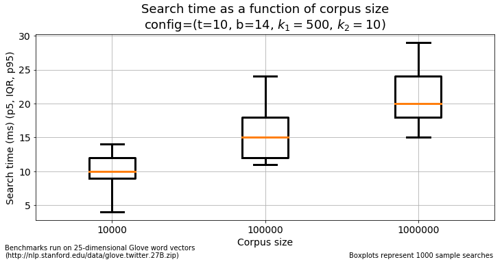
Search for a vector's neighbors: < 500 milliseconds. Search time scales sub-linearly with the size of the corpus.

The corpus vs. search time generally follows a sub-linear pattern like this:

Beyond that, speed is a function of:

The vectors' dimensionality.
The number of tables (a.k.a. hash functions or trees) in the LSH model.
The number of bits in the LSH model's hashes.
The number of approximate neighbors retrieved, k1.
The number of exact neighbors returned, k2.

In the image similarity search engine, you can see that searches against an index of 6.7 million 1000-dimensional vectors rarely exceed 200 milliseconds.

Recall

Recall is defined as the proportion of true nearest neighbors returned for a search and can be evaluated at various values of k2. For example, if you know your application needs to retrieve the top ten most similar items, you should evaluate recall at k2 = 10.

Similar to speed, recall depends on the LSH configuration. Increasing k1 is typically the easiest way to increase recall, but the number of tables and bits also play an important role. Finding a configuration to maximize recall and minimize search time can be considered a form of hyper-parameter optimization.

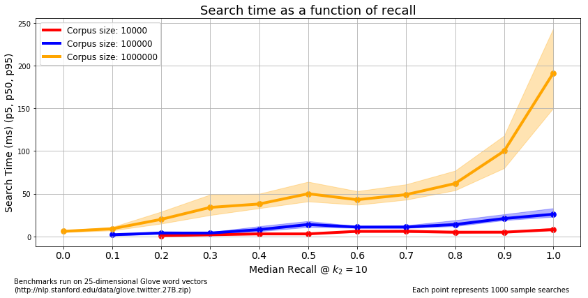
The figure below demonstrates that it is possible to find a configuration with high-recall and low search-time at various corpus sizes. The points plotted represent the "frontier" of recall/search-time. That is, I ran benchmarks on many configurations and chose the configurations with the lowest median search time for each median recall across three corpus sizes.

The table below shows the best configuration for each combination of corpus size, median recall, median search time with a median recall >= 0.5.

	Corpus size	Med. recall	Med. search time	k1	_aknn_nb_tables	_aknn_nb_bits_per_table
0	1000000	1	191	500	200	12
1	1000000	0.9	100	500	100	14
2	1000000	0.8	62	1000	50	16
3	1000000	0.7	49	500	50	16
4	1000000	0.6	43	250	50	16
5	1000000	0.5	50	250	50	19
6	100000	1	26	250	100	12
7	100000	0.9	21	500	50	14
8	100000	0.8	14	250	50	18
9	100000	0.7	11	100	50	14
10	100000	0.6	11	100	50	19
11	100000	0.5	14	500	10	8
12	10000	1	8	100	100	8
13	10000	0.9	5	100	50	12
14	10000	0.8	5	100	50	18
15	10000	0.7	6	250	10	8
16	10000	0.6	6	15	100	18
17	10000	0.5	3	15	50	14

Image Processing Pipeline

Implementation

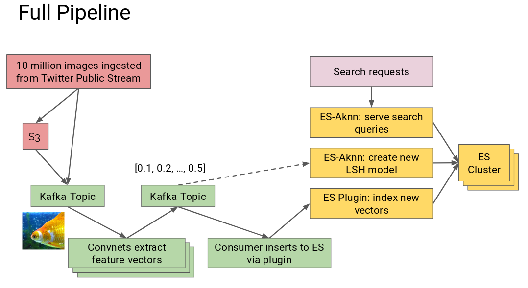
The image processing pipeline consists of the following components, shown in pink and green above:

Python program ingests images from the Twitter public stream and stores in S3.
Python program publishes batches of references to images stored in S3 to a Kafka topic.
Python program consumes batches of image references, computes feature vectors from the images, stores them on S3, publishes references to Kafka. I use the conv_pred layer from Keras pre-trained MobileNet to compute the 1000-dimensional feature vectors.
Python program consumes image features from Kafka/S3 and indexes them in Elasticsearch via EsAknn.

Performance

Image feature extraction is the main bottleneck in this pipeline. It's embarrassingly parallel but still requires thoughtful optimization. In the end I was able to compute:

40 images / node / second on EC2 P2.xlarge (K80 GPU, $0.3/hr spot instance).
33 images / node / second on EC2 C5.9xlarge (36-core CPU, $0.6/hr spot instance).

My first-pass plateaued at about 2 images / node / second. I was able to improve throughput with the following optimizations:

Produce image references to Kafka instead of full images. This allows many workers to download the images in parallel from S3. If you send the full images through Kafka, it quickly becomes a bottleneck.
Workers use thread pools to download images in parallel from S3.
Workers use process pools to crop and resize images for use with Keras.
Workers use the Lycon library for fast image resizing.
Workers use Keras/Tensorflow to compute feature vectors on large batches of images instead of single images. This is a standard deep learning optimization.

Helpful Resources

Here are a handful of resources I found particularly helpful for this project:

Locality Sensitive Hashing lectures by Victor Lavrenko
Elasticsearch Plugin Starter by Alexander Reelsen
Elasticsearch OpenNLP Plugin by Alexander Reelsen
Discussions about similarity search in Elasticsearch: one, two.

mattiasarro/elastik-nearest-neighbors

ElastiK Nearest Neighbors

Overview

Demo

Elasticsearch-Aknn

Usecase

How does it compare to other approximate-nearest-neighbors libraries?

API

Create LSH Model

Index New Vectors

Similarity Search

Implementation

Performance

Speed

Recall

Image Processing Pipeline

Implementation

Performance

Helpful Resources