Authors: Matt Johnson and Scott Linderman
This package combines pyhsmm and pylds to provide simple interfaces for learning and inference in switching linear dynamical systems (SLDS). We support inference via blocked Gibbs sampling, structured mean field, and expectation maximization (EM) for either linear Gaussian or, using pypolyagamma, count observations. The inference algorithms use fast message passing implementations and count observation models additionally use the Pólya-gamma augmentation.
To install pyslds, just run
pip install pyslds
To enable OpenMP support in pypolyagamma, you might want to install it separately following their installation instructions for OpenMP support.
git clone git@github.com:mattjj/pyslds.git
pip install -e pyslds
Switching linear dynamical systems (SLDS) are powerful
models for approximating nonlinear dynamical systems. The basic idea
is to model the data, y_t, as a linear projection of a
low-dimensional latent state, x_t. Moreover, these continuous latent
states co-evolve alongside a discrete latent state, z_t. The
instantaneous discrete state indexes into a set of linear dynamics
parameters. That is, in order to propagate the continuous state forward
one time step, we first sample the next discrete state, then we use
the linear dynamics associated with that discrete state to update the
continuous state. This is summarized with the following dynamics equations:
Here, A_k, Q_k, C_k, and R_k are matrices associated
with discrete state z_t = k, and b_k and d_k are vector
biases associated with these states. While the dynamics are
conditionally linear given the discrete latent state, the composition
of many linear systems is highly nonlinear.
PySLDS exposes a variety of classes for working with linear dynamical systems. For example, the following snippet will generate synthetic data from a random model:
import numpy.random as npr
from pyslds.models import DefaultSLDS

K = 5               # Number of discrete latent states
D_obs = 1           # Observed data dimension
D_latent = 2        # Latent state dimension
D_input = 0         # Exogenous input dimension
T = 2000            # Number of time steps to simulate

true_model = DefaultSLDS(K, D_obs, D_latent, D_input)
inputs = npr.randn(T, D_input)
y, x, z = true_model.generate(T, inputs=inputs)

# Compute the log likelihood of the data with the true params
true_ll = true_model.log_likelihood()
The DefaultSLDS constructor initializes an SLDS with a
random walk dynamics. The outputs are y, a T x D_obs
matrix of observations, and x, a T x D_latent matrix
of continuous latent states, and z, a length-T vector of integers
denoting the discrete latent states.
Now create another SLDS and try to infer the latent states and learn the parameters given the observed data.
# Create a separate model and add the observed data
test_model = DefaultSLDS(K, D_obs, D_latent, D_input)
test_model.add_data(y)

# Run the Gibbs sampler
N_samples = 1000
def update(model):
    model.resample_model()
    return model.log_likelihood()

lls = [update(test_model) for _ in range(N_samples)]
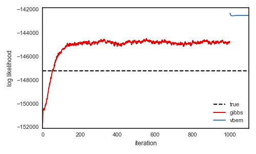
We can plot the log likelihood over iterations to assess the convergence of the sampling algorithm:
# Plot the log likelihoods
plt.figure()
plt.plot([0, N_samples], true_ll * np.ones(2), '--k', label="true")
plt.plot(np.arange(N_samples), lls, color=colors[0], label="test")
plt.xlabel("iteration")
plt.ylabel("training likelihood")
plt.legend(loc="lower right")
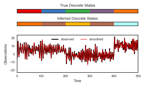
We can also smooth the observations with the test model.
# Smooth the data
smoothed_data = test_model.smooth(data, inputs)

plt.figure()
plt.plot(data, color=colors[0], lw=2, label="observed")
plt.plot(smoothed_data, color=colors[1], lw=1, label="smoothed")
plt.xlabel("Time")
plt.xlim(0, 500)
plt.ylabel("Smoothed Data")
plt.legend(loc="upper center", ncol=2)
This is based on the simple demo in the the examples directory. Check out that folder for demos of other types of inference, as well as examples of how to work with count data and missing observations.


