An implementation of "Joint Training of a Convolutional Network and a Graphical Model for Human Pose Estimation"
This is a TensorFlow implementation of the paper, which became quite influential in the human pose estimation task (~450 citations).
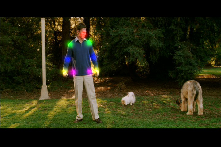
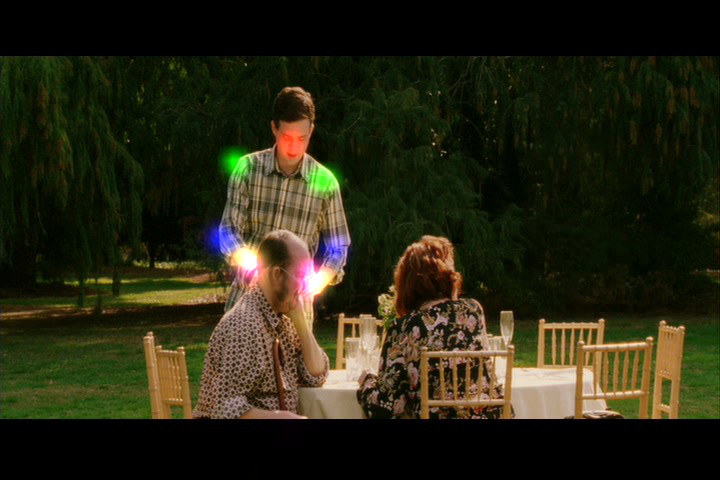
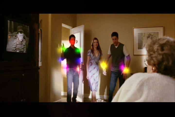
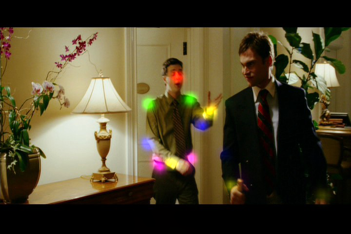
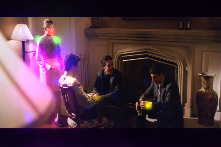
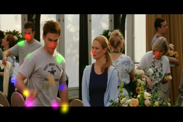
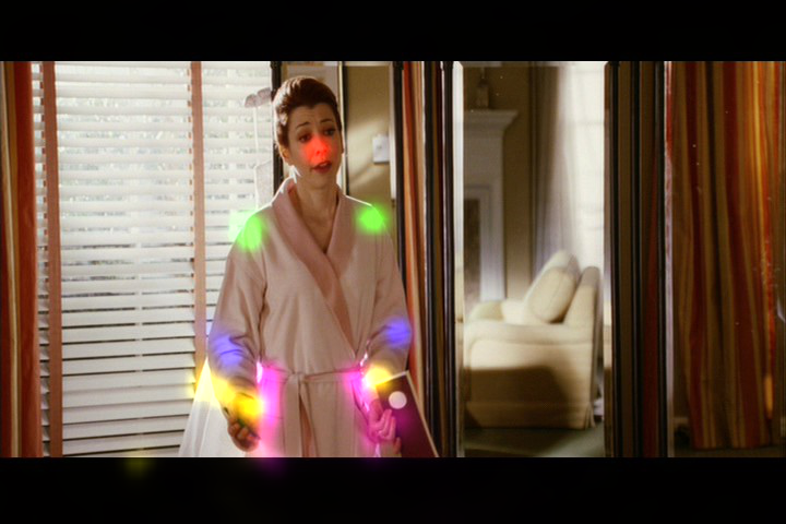
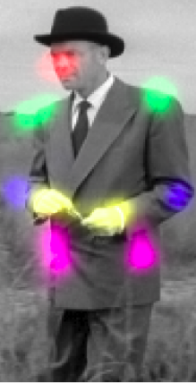
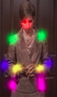
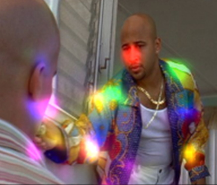
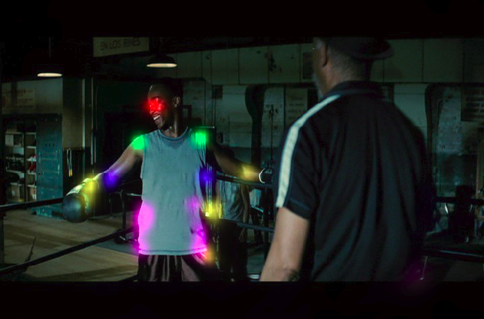
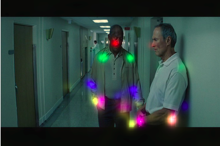
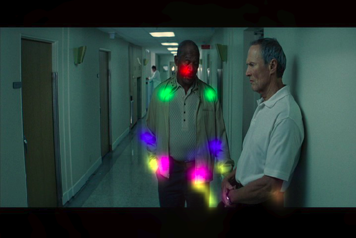
Here are a few examples of joints detection based on FLIC dataset produced with our implementation:
The authors propose a fully-convolutional approach. As input they use multiple images of different resolutions
that aim to capture the spatial context of a different size. These images are processed by a series of 5x5
convolutional and max pooling layers. Then the feature maps from different resolutions are added up, followed
by 2 large 9x9 convolutions. The final layer with 90x60xK feature maps (where K is the number of joints) is our
predicted heat maps. We use then softmax and cross-entropy loss on top of them together with the ground truth
heat maps, which we form by placing a small 3x3 binomial kernel on the actual joint position (see data.py).

Note, that the input resolution 320x240 is not justified at all in the paper, and it is not clear how one can arrive at 98x68 or 90x60 feature maps after 2 max pooling layers. It is quite hard to guess what the authors really did here. Instead we use what makes more sense to us: processing of the full resolution 720x480 images, but first convolution is applied with stride=2, making all dimensions of feature maps comparable in size with what proposed in the paper.
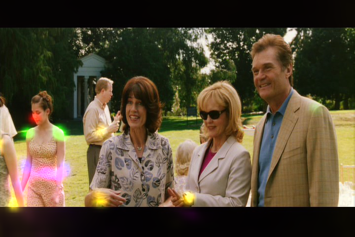
The described part detector already gives good results, however there are also some mistakes that potentially can be ruled out by applying a spatial model. For example, in the third image below there are many false detections of hips (pink color), which clearly do not meet kinematic constraints w.r.t. nose and shoulders that are often detected with very high accuracy.
So the goal is to get rid of such false positives that clearly do not meet kinematic constraints. Traditionally, for such purposes a probabilistic graphical model was used. One of the most popular choices is a tree-structured graphical model, because of the exact inference combined with efficiency due to gaussian pairwise priors, which are most often used. Some approaches combined exact inference with hierarchical structure of a graphical model. Another approaches relied on approximate inference with a loopy graphical model, that allowed to establish connections between symmetrical parts.
An important novelty of this paper is that the spatial model can be modeled as a fully connected graphical
model with parameters that can be trained jointly with the part detector. Thus the graphical model can be
learned from the data, and there is no need to design it for a specific task and dataset, which is a clear
advantage. The schematic description of such spatial model is given below:

We can see a few examples below of how our spatial model trained jointly with the part detector performs compared to the part detector only. On the 1st example we can see that there is a detection of hip of backward facing person. However, this hip does not have any other body parts in its vicinity, so it is ruled out by the spatial model. On the 2nd example there are a few joint detections of person standing on right, and also a minor detection of wrist on the left (small yellow cloud). All of them are ruled out by the spatial model. Note, that there are still some mistakes, but rigorous model evaluation in Section~3 reveals that we indeed get a significant improvement by applying the spatial model.

Surprisingly, we didn't find any implementation in the internet. It can be explained by the fact that the original paper doesn't list any hyperparameters and doesn't provide all necessary implementation details. Thus, it is extremely hard to reproduce, and we decided to add several reasonable modifications from the recent papers to improve the results. However, we kept the architecture of the CNN and the GM without changes.
We introduced the following improvements to the model:
- We train the model 6 times faster by using Batch Normalization, inserted after each activation function, and cross-entropy loss instead of squared loss. Apart from faster training we also achieved better test loss and test detection rate.
- Originally they proposed 3 stages of training: first part detector, then spatial model, and only then the joint training. We could achieve their results with a single stage of the joint training.
- We use an auxiliary classifier on heat maps generated by the part detector. The idea is to make both the part detector and the spatial model to output reasonable heat maps, not only the spatial model. We found this to improve the results.
- We used Adam in order to perform joint training for both part detector and spatial model with a single set of optimizer's hyperparameters. We tried to use SGD with Momentum as suggested in the original paper, but the spatial model requires completely different learning rate and potentially different momentum coefficient. Thus we decided to stick to Adam, which is known to work very well for different functions with the default parameters. Finally, we trained the joint model for 60 epochs with the initial learning rate divided by 2, 5, and 10 after 70%, 80%, and 90% epochs.
- As was mentioned above, we use the whole input images without any special preprocessing. Since the initial image resolution (720x480) is quite big, we apply first convolution with stride 2. In this way we don't discard any information from the dataset (as opposed to 320x240 crop mentioned in the diagram of the CNN, but not explained further in the text).
- We use more advanced data augmentation scheme including horizontal mirroring (with probability 50%), random change of contrast and brightness, random rotation (from -10° to +10°), and random cropping.
- We applied the weight decay only for convolutional filters, since we observed that the highest absolute values of pairwise potentials and biases are quite moderate, and biasing the potentials towards zero is not well motivated.
- We excluded self connections like face->face from the spatial model, which did not make much sense to use and which did not contribute to the final performance.
- We had to adopt the multi-scale evaluation procedure from their previous ICLR paper. This alone gives around +6% detection rate for wrists. We are quite sure that it was actually used in the paper that we implement, however there are no mentions of this procedure. Without this we could not even match the performance of their part detector.
- The previous ICLR paper also mentions quite complicated preprocessing of FLIC training images, which includes manual annotation of the bounding box of the head, and which aims to crop the images in a way that all humans are on the same scale. We tried to apply a procedure similar to this, but it did not lead to successful results. We still think that there was some preprocessing step that could potentially lead to even better results than in our implementation.
- For evaluation and training they flipped left and right joints of backward facing people. We found this only by inspecting their evaluation code.
The evaluation of our model is presented on two plots below, followed by two plots from the original paper.
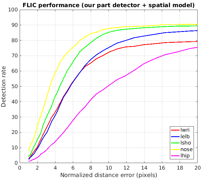
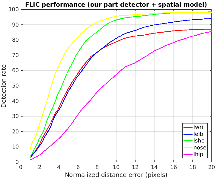
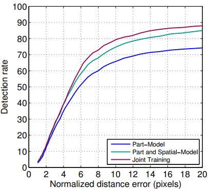
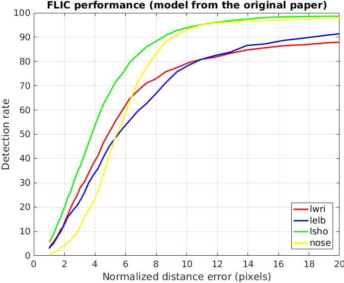
A few observations. Let's consider radius of 10 normalized pixels for the analysis:
- We can observe that our part detector gives +6% accuracy for left wrist (plot 1-1) compared to the original part detector (plot 2-1).
- After applying the spatial model, our model (plot 2-1) has the same accuracy for left wrist and left shoulder (compared to plot 2-2).
- Our spatial model has 3% better accuracy for left elbow and for nose.
- Interestingly, if we consider the accuracy with low radius, our model has much better accuracy for nose, while the original model has much better accuracy for left shoulder. In our opinion, the choice of the loss function and the way one models probabilities (element-wise sigmoid or softmax over a heat map) has the crucial role here.
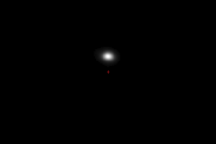
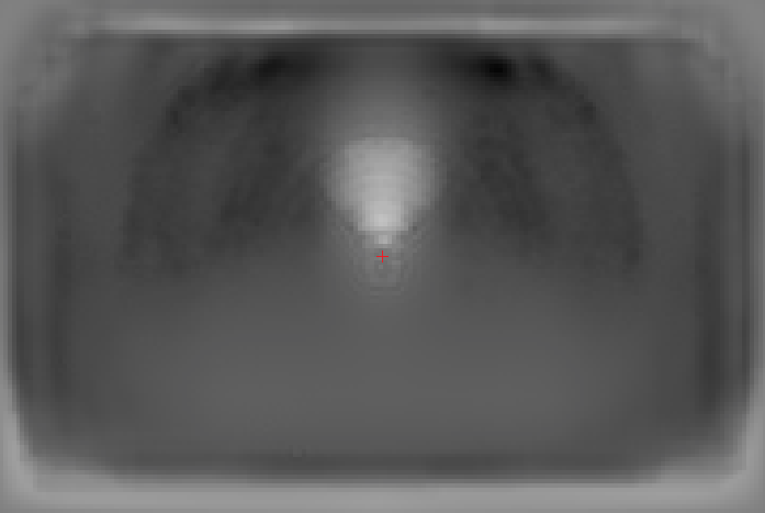
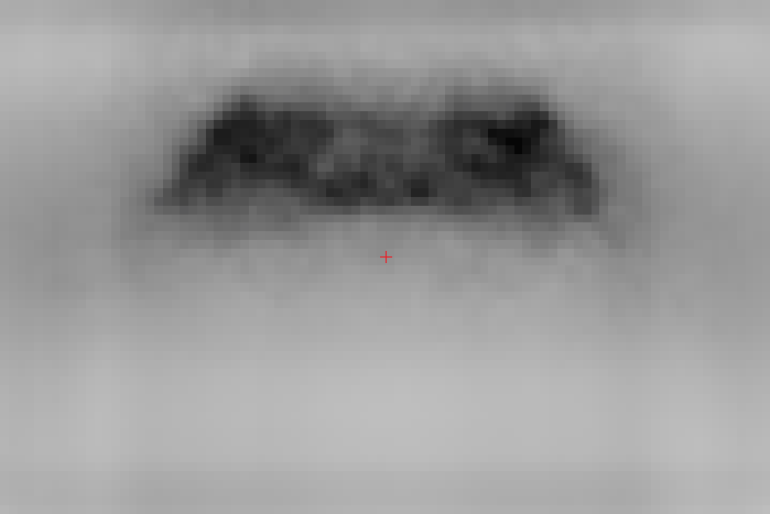
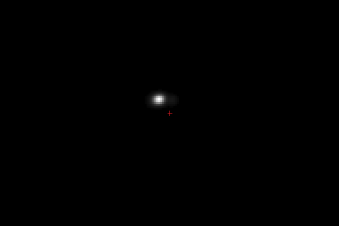
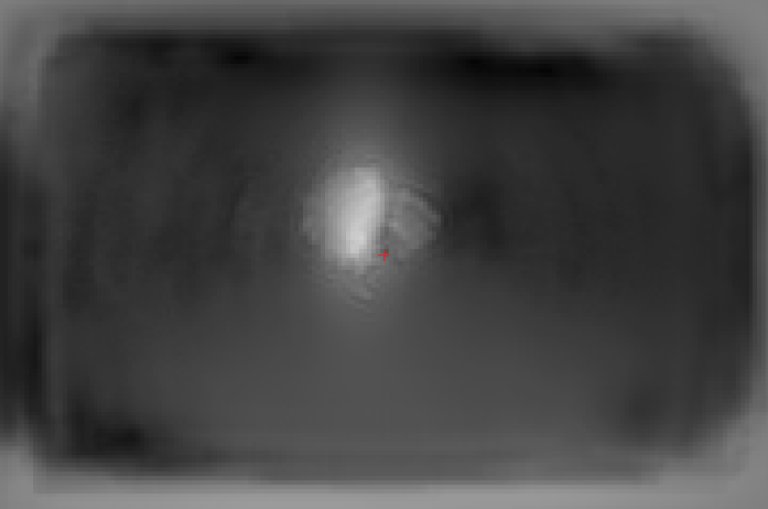
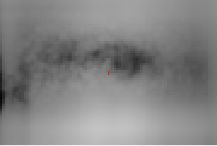
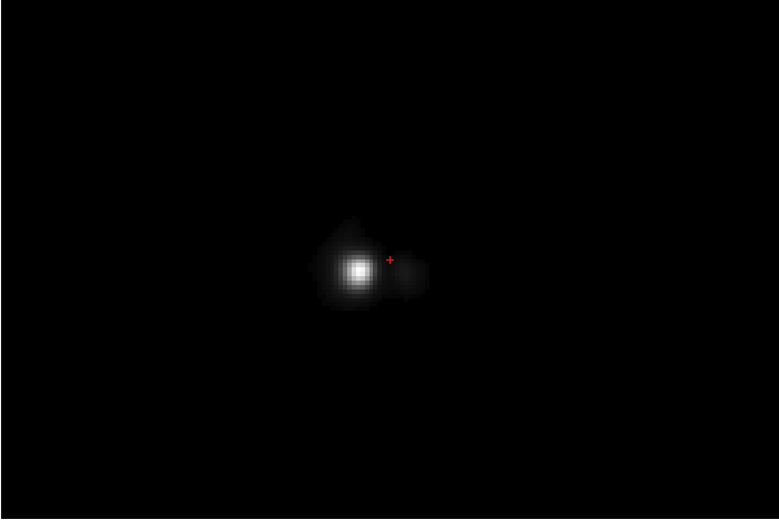
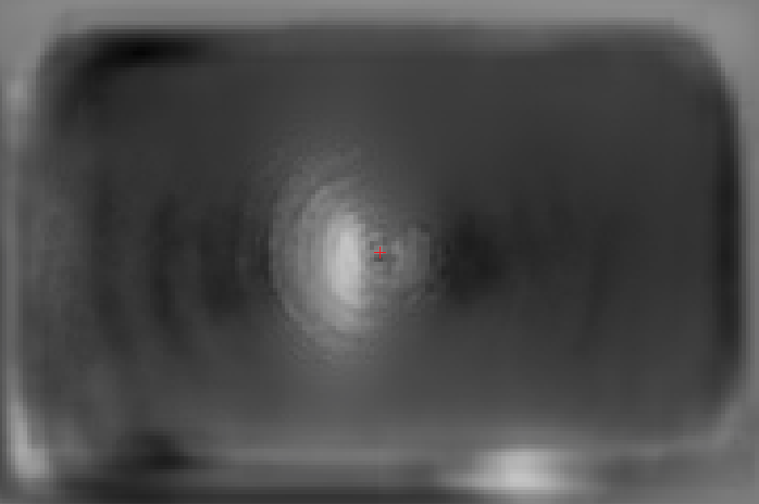
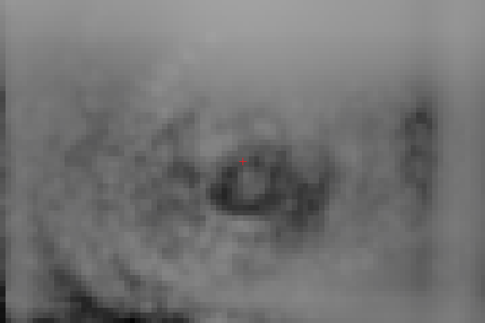
The most interesting question is what kind of parameters for pairwise potentials were learned with backpropagation. We show them below. Please, note that we show pre-softplus values, but after softplus values are obviously similar except negative values. White color denotes high values of parameteres, and dark denotes low values.
| Initialized parameters | Pairwise parameters after 60 epochs | Pairwise biases after 60 epochs |
|---|---|---|
 |
 |
 |
| initial energy of nose|torso | energy nose|torso after 60 epochs | bias nose|torso after 60 epochs |
 |
 |
 |
| initial energy of rsho|torso | energy rsho|torso after 60 epochs | bias rsho|torso after 60 epochs |
 |
 |
 |
| initial energy of relb|torso | energy relb|torso after 60 epochs | bias relb|torso after 60 epochs |
We show only potentials of joints conditioned on torso, because this leads to more distinct patterns. In contrast, e(lhip|rwri) has almost uniform distribution, which means that this connection in a graphical model is redundant.
Our main observations:
- We can notice that for nose and right shoulder we have much more concentrated picture than for right elbow, since there is less ambiguity on where this part can appear relatively to the center of torso.
- Note the circular patterns, especially on e(relb | torso), which are there because of the usage of rotated images (from -10° to +10°) in data augmentation.
- We can also observe that during training all pairwise parameters have changed a lot comparing to the initialization (first column). The borders have grey frames because these values were not actually trained, since border values represent energies for very high displacements of locations between two joints, which are not encountered in the training dataset. So they stayed zeros as they were initialized in the beginning.
- The interpretation of bias terms is rather unclear. Authors claim that their purpose is to correct false negatives produced by the part detector. We cannot confirm this idea by observing the pictures above.
- Download FLIC dataset (FLIC.zip from here).
- Run
python data.pyto process the raw data into x_train_flic.npy, x_test_flic.npy, y_train_flic.npy, y_test_flic.npy. Note, there are 2 varibles:meta_info_file = 'data_FLIC.mat'andimages_dir = './images_FLIC/'that you may need to change.data_FLIC.matis just another name forexamples.matfrom FLIC.zip, andimages_FLIC/is a directory with all the images, which is called justimagesin FLIC.zip. - Run
python pairwise_distr.pyto get file pairwise_distribution.pickle that contains a dictionary of numpy arrays that correspond to empirical histogram of joints displacements. This is a smart initialization of the spatial model described in the paper. - And now you can run the training of the model in a multi-GPU setting:
python main.py --gpus 2 3 --train --data_augm --use_sm --n_epochs=60 --batch_size=14 --optimizer=adam --lr=0.001 --lmbd=0.001
Supported options (or you can simply type python main.py --help):
debug: debug mode means the usage of limited number of train/test data and 4 times less convolutional filter in the part detector.train: True if we want to train the model. False if we just want to evaluate (obviously, best used withrestore=True).gpus: list of GPU IDs to train on. Note, if you have too many GPUs with relatively low batch size, then BatchNorm can be less efficient.restore: True if you want to restore an existing model, name of which should be specified inbest_model_namevariable.use_sm: True if you want ro use the Spatial Model or not.data_augm: True if you want to apply data augmentation.n_epochs: number of epochs.batch_size: batch size. Note, if you are in the multi-GPU setting, then each GPU will receive batch_size / #n_gpus images.optimizer:adamormomentum, both are with default parameters except the learning rate.lr: learning rate.lmbd: coefficient of weight decay, which is applied only to convolutional weights of the part detector.
Note that the script main.py saves tensorboard summaries (folder tb) and model parameters (folder models_ex).
For any questions regarding the code please contact Maksym Andriushchenko (m.my surname@gmail.com). Any suggestions are always welcome.
You can cite the original paper as:
@inproceedings{tompson2014joint,
  title={Joint training of a convolutional network and a graphical model for human pose estimation},
  author={Tompson, Jonathan J and Jain, Arjun and LeCun, Yann and Bregler, Christoph},
  booktitle={Advances in neural information processing systems},
  pages={1799--1807},
  year={2014}
}