Reinforcement Learning for Algorithmic Trading

Getting Started

Python 3.6.5

I would reccomend creating a virtual enviorment to avoid dependancy issues. You can create a virtual enviorment using Virtualenv if you don't already have it installed in your current python interpreter. The current dependancies are in requirements-cpu.txt or gpu equivalent, and can be installed by the following commands.

pip3 install virtualenv
python3 -m virtualenv env

source env/bin/activate

pip install -r requirements-cpu.txt

The equivalent requirements for gpu support are inside requirements-gpu.txt.

Training

We are currently working on optimizing the distribution of funds between two assets. You run python main.py [source type], where the source type(s) are as follows:

markov
- Markov memory 1 and a fixed asset with return rate 0
markov2
- Markov memory 2 and a fixed asset with return rate 0
iid
- IID uniform random variable and a fixed asset with return rate 0
mix
- Markov memory 1 and IID uniform r.v
real
- Real data

This will populate the contents of a Q table and display the result of following the policy obtained over 100 intervals of testing data. An overview of the code architechure is found below.

main.py
- This is where you can specify episodes and initial investment
enviorment.py
- Here you can manipulate paramaters of the trading enviorment such as action space, observation space, reward function and done flag
Q_table.py
- This class defines learning rate, gamma, epsilon parameters and contains choice action and learning methods
utils.py
- A series of methods used to import, generate and manipulate data for training
/Matlab/
- A bunch of matlab scripts that have been used to determine quantizers, empirical distributions and policies.

Q Learning Results

Below are some observations thus far. Each example is derived with an initial investment of $100 for 10 episodes.

IID Source

When the input source is an iid random variable uniformly distributed on [-1,1] with steps of 0.2, the Q table is populated as follows. Note that there is no observation space, as return rates are independent.

Distribution into Source	0%	10%	20%	30%	40%	50%	60%	70%	80%	90%	100%
None	0.013	-0.016	-0.11	-0.038	-0.009	-0.038	0.004	0.001	-0.038	-0.087	-0.123

Which indicates the best option is to invest %0 of capital into the IID stock at any given time.
When the input source is an iid random variable uniformly distributed on [0,0.3], the Q table is populated as follows.

Distribution into Source	0%	10%	20%	30%	40%	50%	60%	70%	80%	90%	100%
None	1923.39	2243.24	2064.73	2121.45	2028.12	2122.95	2088.61	2155.73	2096.5	2124.11	4931.78

Which indicates the best option is to invest all capital into the IID stock at any given time.

Markov Memory 1 Source

Here the input source is markovian with the following transition probabilities.

If the possible return rates for the 3 states are -0.2, 0.0, 0.2 the Q table is populated as follows.

Distribution into Source	0%	10%	20%	30%	40%	50%	60%	70%	80%	90%	100%
Prev Value: 0	218.074	111.159	127.127	105.276	112.809	102.041	98.145	97.792	113.613	95.798	106.162
Prev Value: 0.2	181.137	191.67	261.255	187.992	172.182	179.056	223.266	186.9	182.004	217.171	629.632
Prev Value: -0.2	244.331	58.172	62.42	48.51	56.312	55.855	50.747	63.276	77.343	52.846	55.282

This deduces the policy that, when the previous value is:

0 -> Do not invest
-0.2 -> Do not invest
0.2 -> Invest %100 of capital into stock

If the return rates for the 3 possible states are -0.1, 0, 0.4, the Q table below is produced.

Distribution into Source	0%	10%	20%	30%	40%	50%	60%	70%	80%	90%	100%
Prev Value: -0.1	559.623	62.7048	60.9816	68.2782	61.0308	66.2113	58.6067	56.0653	64.5082	60.6457	56.6935
Prev Value: 0	69.0304	72.4873	64.9642	58.6928	61.7887	561.144	70.8124	69.7554	66.7248	63.1553	64.2676
Prev Value: 0.4	159.824	196.479	200.312	181.142	205.622	200.464	184.247	178.793	196.372	172.393	1281.63

This deduces the policy that, when the previous value is:

0 -> Invest %50 of capital into stock
-0.1 -> Do not invest
0.4 -> Invest %100 of capital into stock
This results are consistend with the optimal investement decision derived in the ./Matlab/ scripts, which yields that the Q-learning is working effectivly.

Using the script ./Matlab/ModelFitting.m the one step transition matrix for IBM computed over the IBM return rates, (discluding the last 1000 samples for testing).

For states x < -.1%, -.1% < x < .1% and x > .1%. We can then enter this transition matrix and states in `utils.py` to generating 5000 samples, and then train the Q learning agent on these samples. Applying the policy obtained from Q-learning, we can then apply it to the testing data for IBM (the last 1000 values).

However, this quantization is generic and randomly chosen. Consider now repeating the experiment, however, we can determine the quantization of our training data using the Lloyd Max algorithm on the real data training set.

Applying this quantiation to `./Matlab/ModelFitting.m` we generate the following transition matrix.

Training a Q agent on the dataset generated according to this empirical distribution and applying the policy obtained to the testing data yeilds the following result.

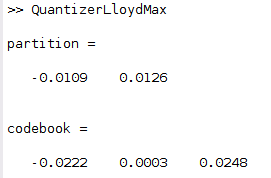
Repeating this experiment with the Microsoft data, we first obtain a Llloyd Max quantizatizer as shown below.

Afterwards we can obtain an empiratical approximation of the 1 step transition matrix according to this quantizer, with respect to the MSFT data discluding the most recent 1000 entries.

Using this quantizer and transition matrix to generate training data for the Q agent, the policies obtained have the following result on our testing data.

Comparing Q Learning Results for Markov Orders

To better understand what markov order (if any) best represents the conditional dependence of past return rates we experiment with manipulating the obsersvations seen by the Q learning agent. To start, we consider the microsoft data. Below is the populated Q table if this stock is treated as iid. Here, the agent has no access to previous return rates so the observation is always the same.

Distribution into Source	0%	10%	20%	30%	40%	50%	60%	70%	80%	90%	100%
None	39.2431	39.5498	39.2918	40.3238	39.5636	48.7792	39.8656	39.8663	39.4475	39.746	39.4284

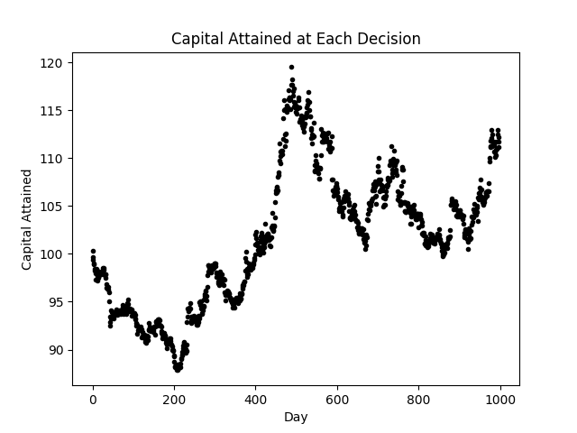
This policy implies investing %90 of assets into the stock for any given time step. Applying such policy over the testing data yeilds.

Now, if we allow the Q learning agent to observe the previous return rate as `-1, 0, 1` correspoding to being in the negative interval, nuetral interval and positive interval as per the uniform quantization over the training data, we observe the following markov order 1 policy from the Q learning agent.

Distribution into Source	0%	10%	20%	30%	40%	50%	60%	70%	80%	90%	100%
Prev "Down"	8.69687	8.416	8.76448	8.32668	8.06351	8.44431	8.61975	19.2718	9.00001	7.86183	7.99984
Prev "Nuetral"	21.6007	21.3949	21.1213	21.2595	21.0212	21.3045	20.5782	21.1772	20.8734	28.6595	21.2023
Prev "Positive"	8.626	8.10509	18.6383	8.12764	8.08328	8.12089	7.71774	8.01588	8.39773	8.66198	8.14364

This markov policy yeilds the following performance over the testing data.

Allowing the Q agent to look at the previous two return rates yeilds the following Q table.

Distribution into Source	0%	10%	20%	30%	40%	50%	60%	70%	80%	90%	100%
Prev Seq: "Down", "Down"	1.46329	1.34375	1.31343	1.51526	1.36004	1.47882	4.51021	1.35624	1.63156	1.34464	1.29957
Prev Seq: "Down", "Nuetral"	4.35364	4.07422	3.88701	4.19443	4.04607	3.83908	4.51836	4.09829	10.6058	3.95363	4.04416
Prev Seq: "Down", "Positive"	1.16335	1.42665	1.21431	1.37276	1.42155	1.41948	1.36941	4.42286	1.15609	1.05923	1.19335
Prev Seq: "Nuetral", "Down"	2.88785	2.68302	3.32496	2.92446	2.70594	2.6983	2.91641	2.71681	7.94342	3.07691	2.84623
Prev Seq: "Nuetral", "Nuetral"	15.2012	15.0627	22.1063	14.9272	14.9772	15.1129	14.9588	14.7254	14.772	15.2999	15.2734
Prev Seq: "Nuetral", "Postive"	7.55047	3.08106	3.07143	3.17324	2.909	3.29652	2.78571	3.24299	3.09982	2.82638	3.24957
Prev Seq: "Positive", "Down"	4.64262	1.45491	1.49116	1.44225	1.37647	1.39101	1.6392	1.17189	1.3111	1.53721	1.38324
Prev Seq: "Positive", "Nuetral"	3.74981	4.25076	4.28741	9.85611	4.12424	4.65483	4.37102	4.29442	3.81727	4.28817	3.76588
Prev Seq: "Positive", "Positive"	1.22974	1.00224	1.16756	1.04358	1.34929	1.13015	1.25551	3.65231	0.896386	1.18419	1.17435

Applying this markov 2 policy to the testing set yeilds

Interestingly engough, the seccond order memory performed worse. This is due to Q learning agent not being able to appropriately explore all states. In order to allow the agent to derive a markov memory 2 policy we must increase the number of training episoides. Conducting the equivilant experiment for the IBM data yeilds the following results. When treated as IID, the following Q table is derived.

Distribution into Source	0%	10%	20%	30%	40%	50%	60%	70%	80%	90%	100%
None	43.8113	43.8479	43.6593	44.0324	44.544	44.5033	43.8169	44.1369	43.9382	54.4591	44.3226

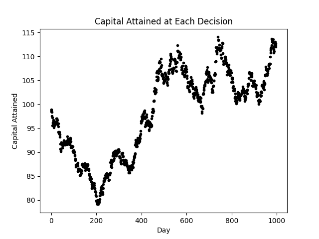
And applying such policy to the testing data yeilds.

Moving to markov memory 1, we obtain the following Q table.

Distribution into Source	0%	10%	20%	30%	40%	50%	60%	70%	80%	90%	100%
Prev "Down"	10.2676	10.2352	11.1674	10.8175	10.6088	11.0861	10.3039	22.9233	9.90889	10.1815	9.52493
Prev "Nuetral"	23.2557	23.2025	23.4107	23.7157	23.1266	23.4601	31.6622	24.0064	22.8477	23.2966	23.6219
Prev "Positive"	7.81495	7.97147	8.75302	8.76693	8.49904	8.13567	8.53647	8.06919	8.06033	8.29538	20.0326

Which yeilds the following testing results.

The difference between the IID test and markov 1 test is that the markov 1 policy seems to be less "risky", it looses less money at the begining of the testing period, however, gains less towards the end. The two policies appear to be very simaler. Moving forward to markov order 2, we obtain the following q table.

Distribution into Source	0%	10%	20%	30%	40%	50%	60%	70%	80%	90%	100%
Prev Seq: "Down", "Down"	2.01617	2.08723	1.95979	6.864	1.78769	1.70395	1.87764	2.22568	1.64296	1.81577	2.00709
Prev Seq: "Down", "Nuetral"	5.53366	5.52372	5.12495	5.09426	12.9182	5.1679	5.40856	4.4439	4.89715	4.97982	5.47335
Prev Seq: "Down", "Positive"	1.18736	1.34069	1.44999	1.51097	1.20899	1.38332	4.57586	1.24534	1.38879	1.46921	1.37788
Prev Seq: "Nuetral", "Down"	3.6141	3.97473	3.66598	3.66956	3.88415	9.45307	3.82271	3.77226	3.98146	3.84407	3.50747
Prev Seq: "Nuetral", "Nuetral"	16.3345	16.0558	15.8404	16.3348	15.6925	16.4471	16.2041	16.3338	16.1826	16.1871	24.4097
Prev Seq: "Nuetral", "Postive"	3.13525	2.72395	2.83029	3.04262	8.08926	2.84946	3.14385	3.14187	2.75471	2.78054	2.84228
Prev Seq: "Positive", "Down"	1.49701	5.84822	1.38522	1.58129	1.71697	1.74671	1.58833	1.83914	1.59212	1.92212	1.68669
Prev Seq: "Positive", "Nuetral"	4.31702	3.85078	10.0363	3.83889	3.75574	3.99425	3.21814	4.12956	3.47642	3.56835	3.76362
Prev Seq: "Positive", "Positive"	1.30869	1.09477	1.28534	1.12935	1.18675	0.935871	0.9024	0.860647	1.13079	1.10643	4.14827

Which yeilds the following performance over out testing period.