dualmarker

Dualmarker is designed for data exploration and hypothesis generation for dual biomarkers. It provides intuitive visualizations and extensive assessment of two marker combinations using logistic regression model for binary outcome (response analysis) and Cox regression for time-to-event outcome (survival analysis).
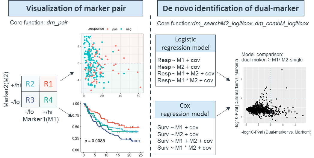
It performs dual marker analysis via two distinct modules:
- One module is evaluation of specific biomarker pair through dm_pair function, which comprehensively reveals the correlation among two markers, response and survival using over 14 sub-plots,such as boxplots, scatterplots, ROCs, and Kaplan-Meier plots.
- Another module is de-novo identification and prioritization of marker2 among candidate markers in combination with known marker1 to predict response and survival through dm_searchM2_cox and dm_searchM2_logit function, its expansion version works for all biomarker combination to prioritize the most significant pair through dm_combM_cox and dm_combM_logit function.
It is applicable for both response and survival analyses and compatible with both continuous and categorical variables. This figure illustrates the framework of this package.

Installation

Install the latest developmental version from GitHub as follow:

if(!require(devtools)) install.packages("devtools")
devtools::install_github("maxiaopeng/dualmarker")

Key functions

Plenty of commands and functions are wrapped into five main functions: dm_pair for visualization and statistics of given dual marker pairs, dm_searchM2_cox and dm_searchM2_logit for de novo identification of novel marker2 to combine with marker1 using Cox survival model and logistic regression model; dm_combM_cox and dm_combM_logit for de novo identification of marker pairs among all dual marker combinations.

dm_pair

dm_pair is the main function for visualization and statistics of one pair of specific biomarkers. It takes the marker1, marker2, covariates (optional), binary outcome(response) or time-to-event outcome(survival) variable as input, and returns list of comprehensive plots (in response.plot, survival.plot object) and statistic results (in response.stats, survival.stats object) from logistic regression for binary outcome(response) and Cox regression for time-to-event outcome(survival) . The result is a list object with the following structure:

response.plot
- boxplot
- scatter.chart
- four.quadrant
- roc
response.stats
- logit
- four.quadrant
  - param
  - stats
survival.plot
- km.m1m2
- scatter.m1m2
- km.dualmarker
- km.dualmarker.facet
- scatter.dualmarker
- four.quadrant
survival.stats
- cox
- four.quadrant
  - param
  - stats

All visualizations are shown in this overall plot

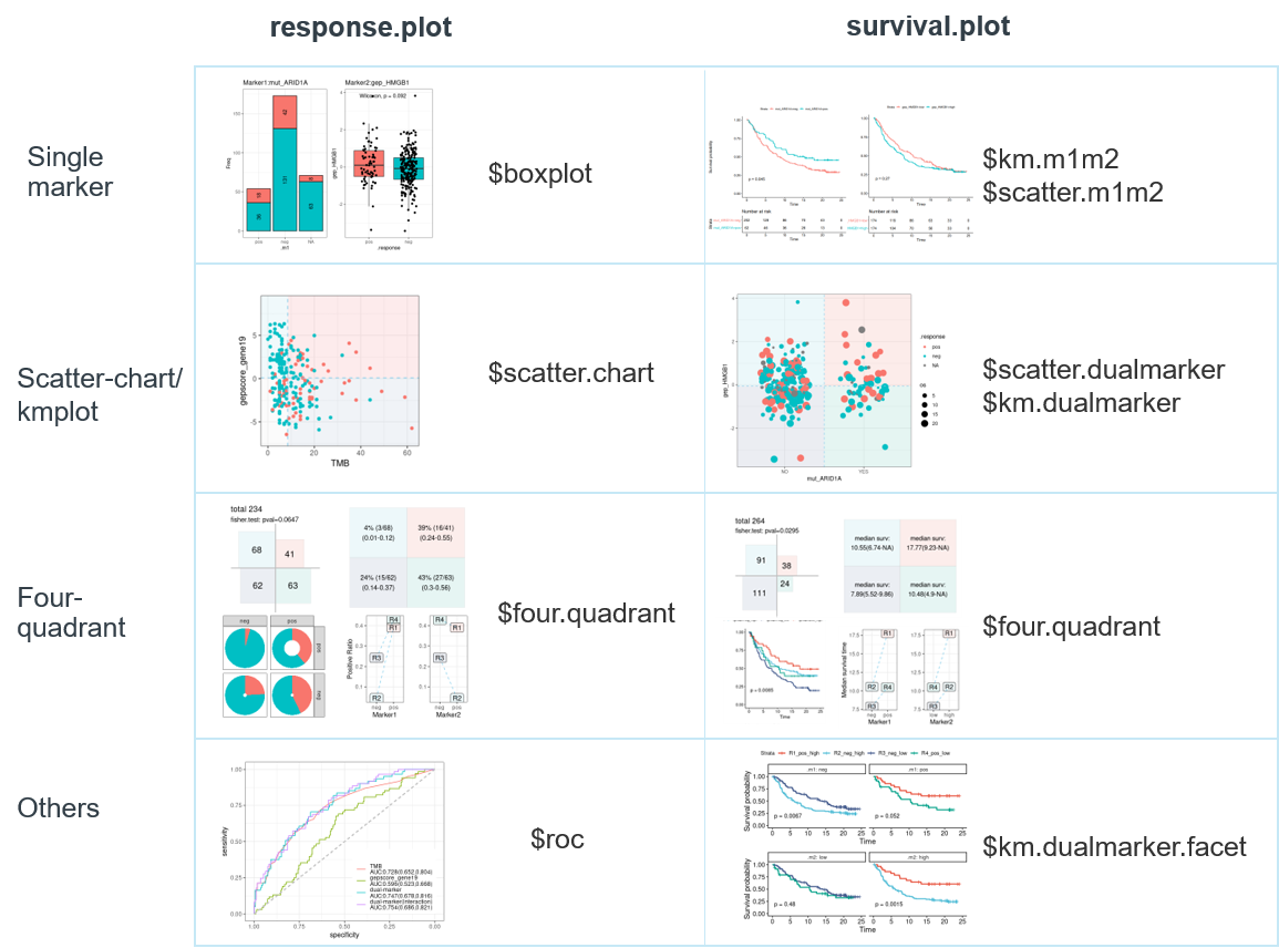
dm_searchM2_cox/logit

The main functions for do novo identification of marker2 from candidates (m2.candidates) to combine with marker1. It takes marker1, and m2.candidates, covariates (optional), binary outcome(response) or time-to-event outcome(survival) variables as input and returns the statistical result of logistic or Cox regression model. Four regression models are built using single marker and dual marker w/ or w/o interaction term:

model1: Surv/Resp ~ marker1 + covariates, labeled as ‘SM1’ for short
model2: Surv/Resp ~ marker2 + covariates , labeled as ‘SM2’ for short
model3: Surv/Resp ~ marker1 + marker2 + covariates, labeled as ‘DM’ for short, i.e. dual-marker
model4: Surv/Resp ~ marker1 * marker2 (with interaction term) + covariates, labeled as ‘DMI’ for short, i.e. dual-marker with interaction

Model comparison is performed between dual-marker and single-marker models by Likihood ratio test(LRT) using anova function. dm_searchM2_topPlot can facilitate the glance of top candidate marker2s for both logistic and Cox regression.
The statistics of regression include the basic information of marker1, marker2, covariates, response, time, event; the estimate and p-values from 4 models, ROC/AUC(for binary outcome), concordant probability estimate(CPE, for survival analysis), AIC, p-values of model comparisons. Users can filter and get interesting dual-marker pairs using the statistics and model performance metrics. Here is an example of logistic regression:

colnames	example values	description
response	binaryResponse	response variable
response_pos	CR, PR	positive response
response_neg	SD, PD	negative response
m1	TMB	marker1 variable
m2	gepscore_TGFb	marker2 variable
covariates	""	covariates variable
cutpoint_m1	NA	cutpoint if m1 is numeric
cutpoint_m2	NA	cutpoint if m2 is numeric
m1_cat_pos	""	positive values if m1 is categorical
m1_cat_neg	""	negative values if m1 is categorical
m2_cat_pos	""	positive values if m2 is categorical
m2_cat_neg	""	negative values if m2 is categorical
SM1_m1_estimate	0.09963989	estimate of marker1 in SM1 model
SM1_m1_p.value	1.395883e-06	pvalue of marker1 in SM1 model
SM2_m2_estimate	-0.1199803	estimate of marker2 in SM2 model
SM2_m2_p.value	0.02516686	pvalue of marker2 in SM2 model
DM_m1_estimate	0.09663392	estimate of marker1 in DM model
DM_m1_p.value	2.582342e-06	pvalue of marker1 in DM model
DM_m2_estimate	-0.08748326	estimate of marker2 in DM model
DM_m2_p.value	0.135587	pvalue of marker2 in DM model
DMI_m1_estimate	0.119926	estimate of marker1 in DMI model
DMI_m1_p.value	1.162081e-06	pvalue of marker1 in DMI model
DMI_m2_estimate	-0.2967303	estimate of marker2 in DMI model
DMI_m2_p.value	0.003635338	pvalue of marker2 in DMI model
DMI_m1:m2_estimate	0.0182465	estimate of interaction m1:m2
DMI_m1:m2_p.value	0.007925505	pvalue of interaction m1:m2
SM1_auc	0.728	AUC of SM1 model
SM2_auc	0.591	AUC of SM2 model
DM_auc	0.747	AUC of DM model
DMI_auc	0.754	AUC of DMI model
SM1_AIC	239.2481	AIC of SM1 model
SM2_AIC	267.3176	AIC of SM2 model
DM_AIC	238.98	AIC of DM model
DMI_AIC	233.9904	AIC of DMI model
pval_SM1_vs_NULL	7.993656e-09	pvalue of SM1-vs-NULL model
pval_SM2_vs_NULL	0.02249407	pvalue of SM2-vs-NULL model
pval_SM1_vs_DM	0.1320594	pvalue of SM1-vs-DM model
pval_SM2_vs_DM	3.630161e-08	pvalue of SM2-vs-DM model
pval_SM1_vs_DMI	0.009765815	pvalue of SM1-vs-DMI model
pval_SM2_vs_DMI	7.84323e-09	pvalue of SM2-vs-DMI model

dm_combM_cox/logit

two functions for de novo identification of biomarker pairs from all dual-marker combinations. They use the similar input and get same output as dm_searchM2_cox/logit.

dataset

We demonstrate the package using Imvigor210 biomarker data. This dataset includes the baseline characterization of PDL1 protein level(IHC), gene expression profiling(GEP) and mutations on 348 advanced UC patients as well as response and Overall survival(OS) data treated by Atezolizumab.
The demographic info, clinical efficacy and biomarker data is stored in clin_bmk_IMvigor210 dataframe, with gene expression variables containing ‘gep_’ prefix, gene signature score variables containing ‘gepscore_’ prefix and mutation variables containing ‘mut_’ prefix. The GEP data and gene signature score is processed according to the IMvigor210CoreBiologies package and gene signature score is calculated using hallmark genesets from MsigDBv7.0 as well as signatures from the IMvigor210CoreBiologies package.

library(dualmarker)
library(stringr)
library(dplyr)

Example1: marker pair of TMB + TGF-beta signature

Here we demonstrate the binary outcome (drug response) analysis of TMB + TGF-beta gene signature(gepscore_TGFb.19gene) using dm_pair function. This pair of biomarker is studied in Nature.2018 Feb 22;554(7693):544-548. The response variable should be dichotomized by setting response.pos and response.neg values.

res.pair <- dm_pair(
   data = clin_bmk_IMvigor210, 
   # response info
   response = "binaryResponse", 
   response.pos = "CR/PR", 
   response.neg = "SD/PD", 
   label.response.pos = "R",
   label.response.neg = "NR",
   # marker1
   marker1 = "TMB", 
   m1.num.cut = "median",  # default median cut for continuous variable
   label.m1 = "TMB",
   label.m1.pos = "TMB_hi",
   label.m1.neg = "TMB_lo",
   # marker2
   marker2 = "gepscore_TGFb.19gene", 
   m2.num.cut = "median", 
   label.m2 = "TGF_beta", 
   label.m2.pos = "TGFb_hi",
   label.m2.neg = "TGFb_lo",
   # others
   na.rm.response = F, # show NA for response variable
   na.rm.marker = F,  # show NA from marker variable
   # palette
   palette.4quadrant = "default", 
   palette.other = "default"
)

plot-1: [response analysis] Single marker
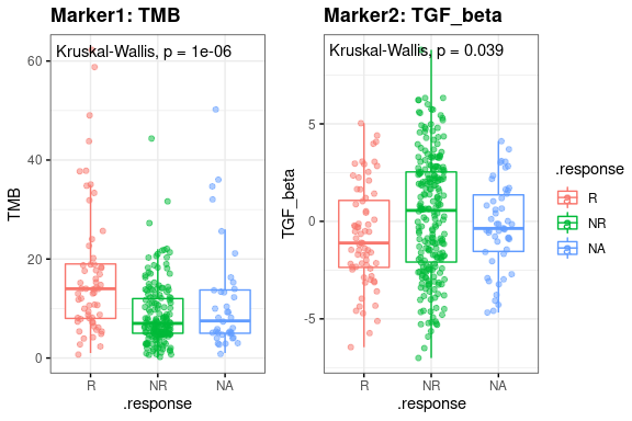
The correlation between single marker and drug response is shown in boxplot, labeled with p-values of Wilcoxon test between positive and negative outcome(response).

res.pair$response.plot$boxplot

plot-2: [response analysis] Scatter chart
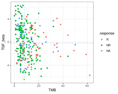
The correlation between marker1, maker2 and drug response is shown in scatter-chart with color indicating response status. If marker1 and/or marker2 is categorical, the jitter plot will be shown.

res.pair$response.plot$scatter.chart

plot-3: [response analysis] Four-quadrant chart
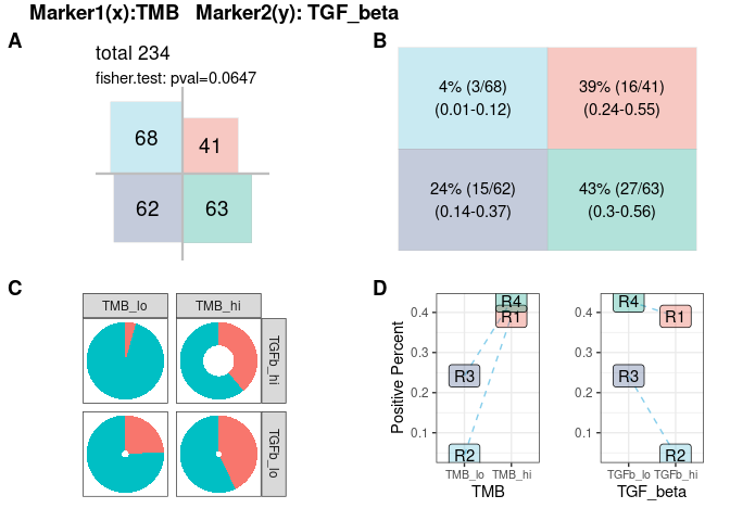
Samples are split into four groups/quadrants(R1-R4), according to cutoffs for continuous markers, default using ‘median’. The independence of each group/quadrant is tested by Fisher exact test. Response rate, sample size and confidence interval are shown in matrix, doughnut chart and line chart. For the doughnut chart, response rate is corresponding to red arc fraction and sample size to width of ring, and the line chart reveals the response rate and potential statistical interaction from two markers if lines are crossed.

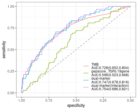
res.pair$response.plot$four.quadrant

plot-4: [response analysis] ROC curve
The single and dual marker prediction of drug response is also shown on ROC curve. Logistics regression model is applied w/ or w/o interaction term between two biomarkers. AUC value and its confidence interval is also drawn on the plot

res.pair$response.plot$roc

plot-5: [survival analysis] survival plot of dual marker
not available here, see Example2
plot-6: [survival analysis] survival plot of dual marker
not available here, see Example2
plot-7: [survival analysis] Four-quadrant chart
not available here, see Example2
stats-1: [response analysis] Four-quadrant statistics
(response.stats)four.quadrant contains four-quadrant statistics of response, in the following 2 objects:
- param contains the information of marker1,marker2, et al.
- stats contains the sample number, response rate and its confidence interval in each quadrant, R1-R4

res.4q <- res.pair$response.stats$four.quadrant
res.4q$param
#> # A tibble: 1 x 7
#>   response    response.pos response.neg m1    m2         cutpoint.m1 cutpoint.m2
#>   <chr>       <chr>        <chr>        <chr> <chr>            <dbl>       <dbl>
#> 1 binaryResp… CR/PR        SD/PD        TMB   gepscore_…           8      -0.172
res.4q$stats
#> # A tibble: 4 x 9
#>   region .m1.level .m2.level n.total n.pos n.neg pct.pos pos.lower95 pos.upper95
#>   <chr>  <chr>     <chr>       <int> <int> <int>   <dbl>       <dbl>       <dbl>
#> 1 R1     pos       pos            41    16    25  0.390      0.242         0.555
#> 2 R2     neg       pos            68     3    65  0.0441     0.00919       0.124
#> 3 R3     neg       neg            62    15    47  0.242      0.142         0.367
#> 4 R4     pos       neg            63    27    36  0.429      0.305         0.560

stats-2: [response analysis] Logistic regression result
Four logistic regression models are built. Model comparison between dual-marker and single-marker models is performed by Likelihood ratio test(LRT) using anova function::
- model1: Resp ~ marker1 + covariates, labeled as ‘M1’ for short
- model2: Resp ~ marker2 + covariates, labeled as ‘M2’ for short
- model3: Resp ~ marker1 + marker2 + covariates, labeled as ‘MD’ for short, i.e. dual-marker
- model4: Resp ~ marker1 * marker2 + covariates (with interaction term), labeled as ‘MDI’ for short, i.e. dual-marker with interaction

Logistic regression models return the following values:

basic parameters: time, event, m1(marker1), m2(marker2), cut point of m1/m2 if m1/m2 are continuous, positive/negative values if m1/m2 is categorical
logistic regression parameters: estimate(weight) and p-value(Wald test) of each predictive variable in model1(SM1), model2(SM2), model3(DM), model4(DMI). ‘MDI_.m1:.m2_estimate’ and ‘MDI_m1:m2_pval’ is estimate and p-value of the interaction term of marker1 and marker2
AIC: AIC of SM1,SM2,DM and DMI models
model comparison: p-values of Likelihood Ratio Test(LRT) for SM1-vs-NULL(null model, no marker), SM2-vs-NULL, SM1-vs-DM, SM2-vs-DM, SM1-vs-DMI, SM2-vs-DMI

dplyr::glimpse(res.pair$response.stats$logit)
#> Rows: 1
#> Columns: 40
#> $ response             <chr> "binaryResponse"
#> $ response_pos         <chr> "CR/PR"
#> $ response_neg         <chr> "SD/PD"
#> $ m1                   <chr> "TMB"
#> $ m2                   <chr> "gepscore_TGFb.19gene"
#> $ covariates           <chr> ""
#> $ cutpoint_m1          <lgl> NA
#> $ cutpoint_m2          <lgl> NA
#> $ m1_cat_pos           <chr> ""
#> $ m1_cat_neg           <chr> ""
#> $ m2_cat_pos           <chr> ""
#> $ m2_cat_neg           <chr> ""
#> $ SM1_m1_estimate      <dbl> 0.09963989
#> $ SM1_m1_p.value       <dbl> 1.395883e-06
#> $ SM2_m2_estimate      <dbl> -0.1199803
#> $ SM2_m2_p.value       <dbl> 0.02516686
#> $ DM_m1_estimate       <dbl> 0.09663392
#> $ DM_m1_p.value        <dbl> 2.582342e-06
#> $ DM_m2_estimate       <dbl> -0.08748326
#> $ DM_m2_p.value        <dbl> 0.135587
#> $ DMI_m1_estimate      <dbl> 0.119926
#> $ DMI_m1_p.value       <dbl> 1.162081e-06
#> $ DMI_m2_estimate      <dbl> -0.2967303
#> $ DMI_m2_p.value       <dbl> 0.003635338
#> $ `DMI_m1:m2_estimate` <dbl> 0.0182465
#> $ `DMI_m1:m2_p.value`  <dbl> 0.007925505
#> $ SM1_auc              <dbl> 0.728
#> $ SM2_auc              <dbl> 0.591
#> $ DM_auc               <dbl> 0.747
#> $ DMI_auc              <dbl> 0.754
#> $ SM1_AIC              <dbl> 239.2481
#> $ SM2_AIC              <dbl> 267.3176
#> $ DM_AIC               <dbl> 238.98
#> $ DMI_AIC              <dbl> 233.9904
#> $ pval_SM1_vs_NULL     <dbl> 7.993656e-09
#> $ pval_SM2_vs_NULL     <dbl> 0.02249407
#> $ pval_SM1_vs_DM       <dbl> 0.1320594
#> $ pval_SM2_vs_DM       <dbl> 3.630161e-08
#> $ pval_SM1_vs_DMI      <dbl> 0.009765815
#> $ pval_SM2_vs_DMI      <dbl> 7.84323e-09

stats-3: [survival analysis] Four-quadrant statistics
not available here, see Example2
stats-4: [survival analysis] Cox regression result
not available here, see Example2

Example2: marker pair of ARID1A mutation + CXCL13 expression

Here we demonstrate the visualization of CXCL13 expression and ARID1A mutation , this biomarker pair is studied by Sci Transl Med. 2020 Jun 17;12(548):eabc4220, we showed the same result here.

res.pair <- dm_pair(
   data = clin_bmk_IMvigor210, 
   # response (optional)
   response = "binaryResponse",
   response.pos = "CR/PR", 
   response.neg = "SD/PD",
   label.response.pos = "R", 
   label.response.neg = "NR",
   # survival info
   time = "os", 
   event = "censOS",
   # marker1
   marker1 = "mut_ARID1A",  
   label.m1 = "ARID1A-mut",
   m1.cat.pos = "YES", 
   m1.cat.neg = "NO",
   label.m1.pos = "Mut", 
   label.m1.neg = "Wt",
   # marker2
   marker2 = "gep_CXCL13",
   m2.num.cut = "median", 
   label.m2 = "CXCL13 expression",
   label.m2.pos = "Hi", 
   label.m2.neg = "Lo",
   # palette
   palette.4quadrant = "jco", # color scheme for four-quadrants
   palette.other = "jco",  # color scheme for others
   # others
   na.rm.response = T, # show NA in response variable
   na.rm.marker = T # show NA in biomarker variable: mut_ARID1A, gep_CXCL13
)

plot-1: [response analysis] Single marker
Not shown here, see Example1
plot-2: [response analysis] Scatter chart
Not shown here, see Example1
plot-3: [response analysis] Four-quadrant chart
Not shown here, see Example1
plot-4: [response analysis] ROC curve
Not shown here, see Example1
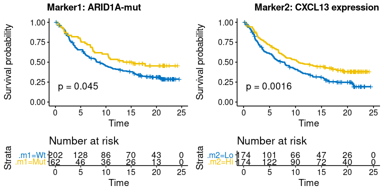
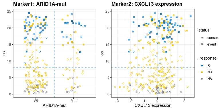
plot-5: [survival analysis] survival plot of single marker
- survival.plot$km.m1m1: KMplot of marker1 and marker2 on two parallel sub-plots
- survival.plot$scatter.m1m2: scatter-plot of survival time(y-axis) and marker1/marker2(x-axis) on two parallel sub-plots, response status(if provided) is shown as color. Nominal survival time is shown and labeled with different shape for the censored data point.

res.pair$survival.plot$km.m1m2

res.pair$survival.plot$scatter.m1m2

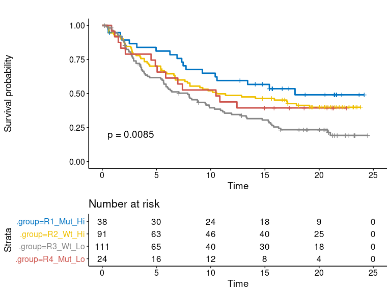
plot-6: [survival analysis] survival plot of dual marker
- km.dualmarker: KMplot of dual marker, corresponding to four quadrants in the scatter plot scenario.
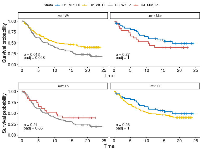
- km.dualmarker.facet: conditional KMplot of dual marker. The conditional KMplot represents the survival curve of marker1 on condition of marker2-level (+/hi or -/lo), and marker2 on condition of marker1 level. It reveals the association between survival and marker1 on the context of marker2 level and vice verse. P-values of log-rank test and adjusted p-values by ‘Bonferroni’ method are shown on each sub-plot.
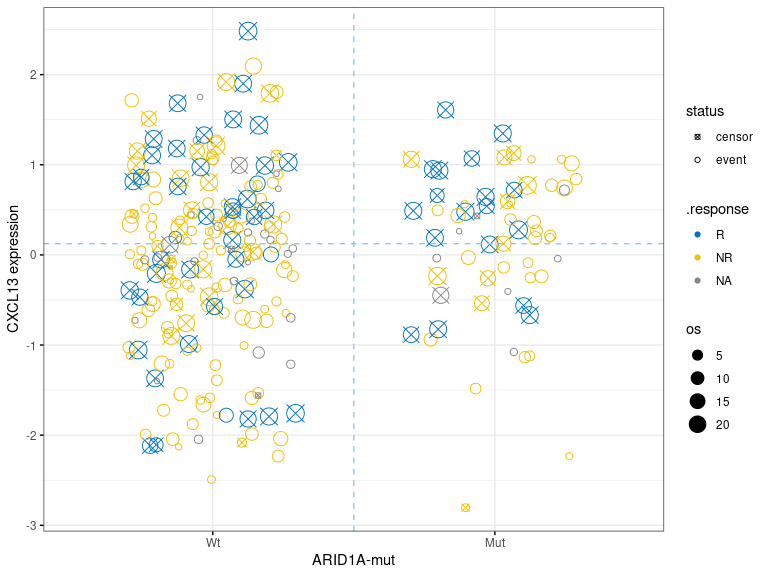
- scatter.dualmarker: scatter-plot of marker1 and marker2 with survival time shown as the size of dot and response (if provided) as color. Nominal survival time is shown and labeled with different shape for the censored data point.

res.pair$survival.plot$km.dualmarker

res.pair$survival.plot$km.dualmarker.facet

res.pair$survival.plot$scatter.dualmarker

plot-7: [survival analysis] Four-quadrant chart
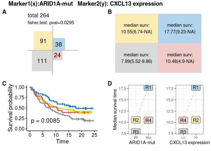
Like response analysis, four-quadrant plots for survival also contains 4 sub-figures.
1. Area proportion chart: shows the sample size in each quadrant, this chart may be different from counterpart in response analysis owning to different missing samples of survival and response data.
2. Statistic matrix: median survival time and confidence interval
3. KMplot of four quadrants
4. Line chart of median survival time for each quadrant

res.pair$survival.plot$four.quadrant

stats-1: [response analysis] Four-quadrant statistics
not shown here, see Example1
stats-2: [response analysis] Logistic regression results
not shown here, see Example1
stats-3: [survival analysis] Four-quadrant statistics
(survival.stats)four.quadrant contains four-quadrant statistics of survival in the following 2 objects:
- param contains the note of marker1,marker2, cutoff methods et al.
- stats contains the sample number, median survival and confidence interval in each quadrant, R1-R4

stats.4q <- res.pair$survival.stats$four.quadrant
stats.4q$param
#> # A tibble: 1 x 10
#>   time  event marker1 marker2 cutpoint.m1 m1.cat.pos m1.cat.neg cutpoint.m2
#>   <chr> <chr> <chr>   <chr>   <lgl>       <chr>      <chr>            <dbl>
#> 1 os    cens… mut_AR… gep_CX… NA          YES        NO               0.124
#> # … with 2 more variables: m2.cat.pos <chr>, m2.cat.neg <chr>
stats.4q$stats
#> # A tibble: 4 x 8
#>   .quadrant .m1   .m2   records events median `0.95LCL` `0.95UCL`
#>   <fct>     <fct> <fct>   <dbl>  <dbl>  <dbl>     <dbl>     <dbl>
#> 1 R1        Mut   Hi         38     18  17.8       9.23     NA   
#> 2 R2        Wt    Hi         91     53  10.5       6.74     NA   
#> 3 R3        Wt    Lo        111     82   7.89      5.52      9.86
#> 4 R4        Mut   Lo         24     14  10.5       4.90     NA

stats-4: [survival analysis] Cox regression result
Like binary outcome (response) analysis, four Cox regression models are built. Model comparison between dual-marker and single-marker models is performed by Likelihood ratio test(LRT) using anova function:
- model1: Surv ~ marker1 + covariates, labeled as ‘SM1’ for short
- model2: Surv ~ marker2 + covariates, labeled as ‘SM2’ for short
- model3: Surv ~ marker1 + marker2 + covariates, labeled as ‘DM’ for short, i.e. dual-marker
- model4: Surv ~ marker1 * marker2 + covariates (with interaction term), labeled as ‘DMI’ for short, i.e. dual-marker with interaction

Cox regression models return the following values:

basic parameters: time, event, m1(marker1), m2(marker2), cut point of m1/m2 if m1/m2 are continuous, positive/negative values if m1/m2 is categorical
Cox regression parameters: estimate(weight) and p-value(Wald test) of each predictive variable in model1(SM1), model2(SM2), model3(DM), model4(DMI). ‘DMI_m1:m2_estimate’ and ‘DMI_m1:m2_pval’ is estimate and p-value of the interaction term of marker1 and marker2.
AIC: AIC of SM1, SM2, DM, DMI model
CPE: concordant probability estimate to evaluate the performance of Cox model using CPE package
model comparison: p-values of Likelihood Ratio Test(LRT) for SM1-vs-NULL(R ~ 1, no marker), SM2-vs-NULL, SM1-vs-MD, SM2-vs-DM, SM1-vs-DMI, SM2-vs-DMI

dplyr::glimpse(res.pair$survival.stats$cox)
#> Rows: 1
#> Columns: 39
#> $ time                 <chr> "os"
#> $ even                 <chr> "censOS"
#> $ m1                   <chr> "mut_ARID1A"
#> $ m2                   <chr> "gep_CXCL13"
#> $ covariates           <chr> ""
#> $ cutpoint_m1          <lgl> NA
#> $ cutpoint_m2          <lgl> NA
#> $ m1_cat_pos           <chr> "YES"
#> $ m1_cat_neg           <chr> "NO"
#> $ m2_cat_pos           <chr> ""
#> $ m2_cat_neg           <chr> ""
#> $ SM1_m1_estimate      <dbl> -0.3931839
#> $ SM1_m1_p.value       <dbl> 0.04572493
#> $ SM2_m2_estimate      <dbl> -0.2869317
#> $ SM2_m2_p.value       <dbl> 0.0001590714
#> $ DM_m1_estimate       <dbl> -0.3134224
#> $ DM_m1_p.value        <dbl> 0.1149989
#> $ DM_m2_estimate       <dbl> -0.2676217
#> $ DM_m2_p.value        <dbl> 0.0004277342
#> $ DMI_m1_estimate      <dbl> -0.3045374
#> $ DMI_m1_p.value       <dbl> 0.1233496
#> $ DMI_m2_estimate      <dbl> -0.2463571
#> $ DMI_m2_p.value       <dbl> 0.002164497
#> $ `DMI_m1:m2_estimate` <dbl> -0.1938994
#> $ `DMI_m1:m2_p.value`  <dbl> 0.4121259
#> $ SM1_AIC              <dbl> 1695.692
#> $ SM2_AIC              <dbl> 1686.086
#> $ DM_AIC               <dbl> 1685.451
#> $ DMI_AIC              <dbl> 1686.794
#> $ SM1_CPE              <dbl> 0.535011
#> $ SM2_CPE              <dbl> 0.5757988
#> $ DM_CPE               <dbl> 0.5834954
#> $ DMI_CPE              <dbl> 0.587801
#> $ pval_SM1_vs_NULL     <dbl> 0.03779216
#> $ pval_SM2_vs_NULL     <dbl> 0.0001907733
#> $ pval_SM1_vs_DM       <dbl> 0.0004674887
#> $ pval_SM2_vs_DM       <dbl> 0.1044939
#> $ pval_SM1_vs_DMI      <dbl> 0.001582535
#> $ pval_SM2_vs_DMI      <dbl> 0.1928236

Example3: search GEP candidates marker2 to combine with mut_ARID1A for survival analysis

Search among gene expression candidates to combine with ARID1A mutation using dm_searchM2_cox

m2.candidates <- stringr::str_subset(colnames(clin_bmk_IMvigor210),"gep_")
res.m2.cox <- dm_searchM2_cox(
   data = clin_bmk_IMvigor210, 
   # survival
   time = "os", 
   event = "censOS",
   # marker1
   marker1 = "mut_ARID1A", 
   m1.binarize = T, 
   m1.cat.pos = "YES", 
   m1.cat.neg = "NO", 
   # marker2
   m2.candidates = m2.candidates, 
   m2.binarize = F, # as continuous variables
   p.adjust.method = "BH"
)

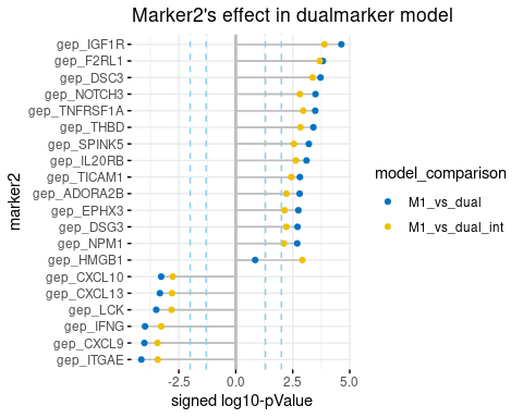
Glance of the top candidates gene: dm_searchM2_topPlot takes the result of either dm_searchM2_cox or dm_searchM2_logit as input, and returns following figures:

$m2_effect dot-chart showing top significant marker2s using model comparison dual-vs-marker1
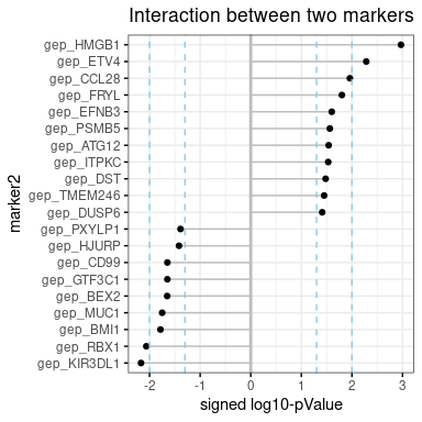
$interact dot-chart showing top significant marker2s having statistical interaction with marker1
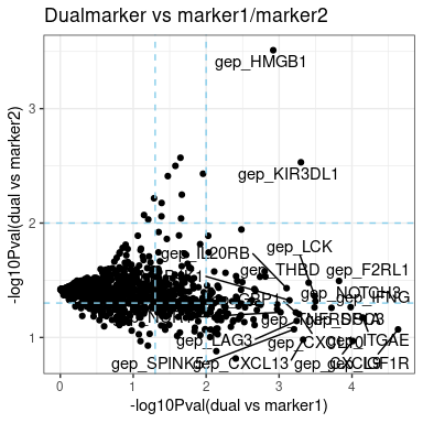
$m1_m2_effect scatter-plot showing log10-p-value of all marker2s in model comparison of dual-vs-marker1 and dual-vs-marker2

plot.m2.cox <- dm_searchM2_topPlot(res.m2.cox, top.n = 20, 
                                   show.padj = F, palette = "jco")

plot-1: marker2 effect
‘m2_effect’ is dot-chart, showing the top significant marker2s, whose introduction to dual-maker model(w/ or w/o interaction) significantly increase the prediction of survival or response. Likelihood ratio test(LRT) is carried out to compare dual-marker model and marker1 single model, the signed log10-pValue is shown on x-axis, and ‘sign’ indicates the effect direction of marker2(single marker) to survival. i.e. genes with negative values on the left are positive survival predictors.

plot.m2.cox$m2_effect

plot-2: marker2’s interaction
‘interaction’ is dot-chart, showing the top significant marker2s, which has statistical interaction with marker1. Signed log10-pValue is shown like ‘m2_effect’

plot.m2.cox$interact

plot-3: m1 and m2 effect
‘m1_m2_effect’ is scatter-plot, showing the -log10-pValue of model comparison, i.e. dual-vs-marker1 and dual-vs-marker2. Dual model that superior to both marker1 and marker2 single marker model is preferred, located top-right on the figure.

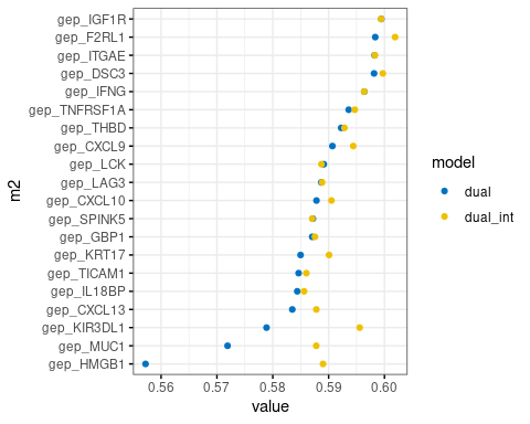
plot.m2.cox$m1_m2_effect

plot-4: CPE ‘CPE’ is concordant probability estimate to evaluate the performance of Cox model using CPE package

plot.m2.cox$CPE

stats: cox result
this shows the same values with res_pair(survival.stats)cox or res_pair(response.stats)logit

dplyr::glimpse(res.m2.cox)
#> Rows: 1,268
#> Columns: 52
#> $ time                 <chr> "os", "os", "os", "os", "os", "os", "os", "os", …
#> $ even                 <chr> "censOS", "censOS", "censOS", "censOS", "censOS"…
#> $ m1                   <chr> "mut_ARID1A", "mut_ARID1A", "mut_ARID1A", "mut_A…
#> $ m2                   <chr> "gep_ADA", "gep_AKT3", "gep_CD24", "gep_BCL2L11"…
#> $ covariates           <chr> "", "", "", "", "", "", "", "", "", "", "", "", …
#> $ cutpoint_m1          <lgl> NA, NA, NA, NA, NA, NA, NA, NA, NA, NA, NA, NA, …
#> $ cutpoint_m2          <lgl> NA, NA, NA, NA, NA, NA, NA, NA, NA, NA, NA, NA, …
#> $ m1_cat_pos           <chr> "YES", "YES", "YES", "YES", "YES", "YES", "YES",…
#> $ m1_cat_neg           <chr> "NO", "NO", "NO", "NO", "NO", "NO", "NO", "NO", …
#> $ m2_cat_pos           <chr> "", "", "", "", "", "", "", "", "", "", "", "", …
#> $ m2_cat_neg           <chr> "", "", "", "", "", "", "", "", "", "", "", "", …
#> $ SM1_m1_estimate      <dbl> -0.3931839, -0.3931839, -0.3931839, -0.3931839, …
#> $ SM1_m1_p.value       <dbl> 0.04572493, 0.04572493, 0.04572493, 0.04572493, …
#> $ SM1_m1_p.adj         <dbl> 0.04572493, 0.04572493, 0.04572493, 0.04572493, …
#> $ SM2_m2_estimate      <dbl> 0.020472278, -0.088602489, -0.040055394, -0.1144…
#> $ SM2_m2_p.value       <dbl> 0.7921732808, 0.2316870325, 0.5845798870, 0.1387…
#> $ SM2_m2_p.adj         <dbl> 0.90686960, 0.48881723, 0.79339732, 0.37478179, …
#> $ DM_m1_estimate       <dbl> -0.3925669, -0.3902232, -0.3992445, -0.3964988, …
#> $ DM_m1_p.value        <dbl> 0.04608730, 0.04740445, 0.04273637, 0.04396925, …
#> $ DM_m1_p.adj          <dbl> 0.07226057, 0.07226057, 0.07226057, 0.07226057, …
#> $ DM_m2_estimate       <dbl> 0.018169157, -0.086696989, -0.048006083, -0.1165…
#> $ DM_m2_p.value        <dbl> 0.815536324, 0.243180093, 0.514144401, 0.1321049…
#> $ DM_m2_p.adj          <dbl> 0.92247998, 0.51861521, 0.75506892, 0.39294519, …
#> $ DMI_m1_estimate      <dbl> -0.4642526, -0.3999853, -0.4101674, -0.3948740, …
#> $ DMI_m1_p.value       <dbl> 0.02572344, 0.04411029, 0.03869969, 0.04542806, …
#> $ DMI_m1_p.adj         <dbl> 0.08066473, 0.08066473, 0.08066473, 0.08066473, …
#> $ DMI_m2_estimate      <dbl> 0.094208982, -0.069846691, -0.092351419, -0.1520…
#> $ DMI_m2_p.value       <dbl> 0.284405899, 0.402004262, 0.263768116, 0.0785384…
#> $ DMI_m2_p.adj         <dbl> 0.60572337, 0.72716320, 0.58779960, 0.33195570, …
#> $ `DMI_m1:m2_estimate` <dbl> -0.37225167, -0.08245620, 0.22222076, 0.17555057…
#> $ `DMI_m1:m2_p.value`  <dbl> 0.05473952, 0.65399403, 0.23758675, 0.35539251, …
#> $ `DMI_m1:m2_p.adj`    <dbl> 0.9961319, 0.9961319, 0.9961319, 0.9961319, 0.99…
#> $ SM1_AIC              <dbl> 1695.692, 1695.692, 1695.692, 1695.692, 1695.692…
#> $ SM2_AIC              <dbl> 1699.937, 1698.583, 1699.707, 1697.803, 1697.684…
#> $ DM_AIC               <dbl> 1697.637, 1696.336, 1697.266, 1695.415, 1695.912…
#> $ DMI_AIC              <dbl> 1695.951, 1698.136, 1697.843, 1696.573, 1697.739…
#> $ SM1_CPE              <dbl> 0.535011, 0.535011, 0.535011, 0.535011, 0.535011…
#> $ SM2_CPE              <dbl> 0.5059344, 0.5255417, 0.5106205, 0.5308784, 0.53…
#> $ DM_CPE               <dbl> 0.5386091, 0.5507807, 0.5433692, 0.5559563, 0.55…
#> $ DMI_CPE              <dbl> 0.5580672, 0.5493288, 0.5512611, 0.5600019, 0.55…
#> $ pval_SM1_vs_NULL     <dbl> 0.03779216, 0.03779216, 0.03779216, 0.03779216, …
#> $ padj_SM1_vs_NULL     <dbl> 0.03779216, 0.03779216, 0.03779216, 0.03779216, …
#> $ pval_SM2_vs_NULL     <dbl> 0.792048437, 0.232822940, 0.584731219, 0.1377636…
#> $ padj_SM2_vs_NULL     <dbl> 0.90684524, 0.48877399, 0.79468294, 0.37566516, …
#> $ pval_SM1_vs_DM       <dbl> 0.815428198, 0.244342092, 0.514221058, 0.1313353…
#> $ padj_SM1_vs_DM       <dbl> 0.92235768, 0.52008877, 0.75466702, 0.39462852, …
#> $ pval_SM2_vs_DM       <dbl> 0.03812741, 0.03933856, 0.03508215, 0.03618768, …
#> $ padj_SM2_vs_DM       <dbl> 0.06163704, 0.06163704, 0.06163704, 0.06163704, …
#> $ pval_SM1_vs_DMI      <dbl> 0.154071909, 0.459326828, 0.396740154, 0.2102864…
#> $ padj_SM1_vs_DMI      <dbl> 0.5613885, 0.7924169, 0.7408932, 0.6386168, 0.73…
#> $ pval_SM2_vs_DMI      <dbl> 0.01844880, 0.10824010, 0.05327299, 0.07316198, …
#> $ padj_SM2_vs_DMI      <dbl> 0.1545506, 0.1545506, 0.1545506, 0.1545506, 0.15…

Top 10 dual marker pairs with the highest concordant probability(CPE)

res.m2.cox %>% 
   dplyr::arrange(desc(DM_CPE)) %>% 
   dplyr::select(m1, m2, DM_CPE) %>%
   head(10) %>% 
   knitr::kable()

m1	m2	DM_CPE
mut_ARID1A	gep_IGF1R	0.5994349
mut_ARID1A	gep_F2RL1	0.5983506
mut_ARID1A	gep_ITGAE	0.5982278
mut_ARID1A	gep_DSC3	0.5981378
mut_ARID1A	gep_IFNG	0.5963877
mut_ARID1A	gep_TNFRSF1A	0.5935954
mut_ARID1A	gep_THBD	0.5922490
mut_ARID1A	gep_CXCL9	0.5906786
mut_ARID1A	gep_LCK	0.5891381
mut_ARID1A	gep_LAG3	0.5886844

Example4: evaluation for all combinations

dm_combM_logit and dm_combM_cox will evaluate all combinations of dual-markers.Searching all biomarker pairs is time-consuming for thousands of gene expression biomarker. Here we demonstrate with only 4 biomarkers.

m.candidates <- c("TMB", "gep_CD274","gep_CXCL13", "gepscore_TGFb.19gene", "mut_ARID1A")
res.combM.logit <- dm_combM_logit(
   data = clin_bmk_IMvigor210, 
   response = "binaryResponse", 
   response.pos = "CR/PR",
   response.neg = "SD/PD", 
   candidates = m.candidates,
   m.binarize = F # don't dichotomize marker
   )

glimpse of the result

dplyr::glimpse(res.combM.logit)
#> Rows: 10
#> Columns: 61
#> $ response                <chr> "binaryResponse", "binaryResponse", "binaryRe…
#> $ response_pos            <chr> "CR/PR", "CR/PR", "CR/PR", "CR/PR", "CR/PR", …
#> $ response_neg            <chr> "SD/PD", "SD/PD", "SD/PD", "SD/PD", "SD/PD", …
#> $ m1                      <chr> "TMB", "TMB", "TMB", "TMB", "gep_CD274", "gep…
#> $ m2                      <chr> "gep_CD274", "gep_CXCL13", "gepscore_TGFb.19g…
#> $ covariates              <chr> "", "", "", "", "", "", "", "", "", ""
#> $ cutpoint_m1             <lgl> NA, NA, NA, NA, NA, NA, NA, NA, NA, NA
#> $ cutpoint_m2             <lgl> NA, NA, NA, NA, NA, NA, NA, NA, NA, NA
#> $ m1_cat_pos              <chr> "", "", "", "", "", "", "", "", "", ""
#> $ m1_cat_neg              <chr> "", "", "", "", "", "", "", "", "", ""
#> $ m2_cat_pos              <chr> "", "", "", "", "", "", "", "", "", ""
#> $ m2_cat_neg              <chr> "", "", "", "", "", "", "", "", "", ""
#> $ SM1_m1_estimate         <dbl> 0.09963989, 0.09963989, 0.09963989, 0.0940112…
#> $ SM1_m1_p.value          <dbl> 1.395883e-06, 1.395883e-06, 1.395883e-06, 3.9…
#> $ SM1_m1_p.adj            <dbl> 4.652943e-06, 4.652943e-06, 4.652943e-06, 9.8…
#> $ SM2_m2_estimate         <dbl> 0.1867642, 0.3217637, -0.1199803, NA, 0.33410…
#> $ SM2_m2_p.value          <dbl> 0.20250772, 0.04076421, 0.02516686, NA, 0.020…
#> $ SM2_m2_p.adj            <dbl> 0.20250772, 0.04891706, 0.03775028, NA, 0.037…
#> $ DM_m1_estimate          <dbl> 0.09848988, 0.09676696, 0.09663392, 0.0941872…
#> $ DM_m1_p.value           <dbl> 2.080848e-06, 3.154783e-06, 2.582342e-06, 6.5…
#> $ DM_m1_p.adj             <dbl> 1.051594e-05, 1.051594e-05, 1.051594e-05, 1.6…
#> $ DM_m2_estimate          <dbl> 0.10743248, 0.23572985, -0.08748326, NA, 0.32…
#> $ DM_m2_p.value           <dbl> 0.503579159, 0.162771037, 0.135586952, NA, 0.…
#> $ DM_m2_p.adj             <dbl> 0.503579159, 0.195325245, 0.195325245, NA, 0.…
#> $ DMI_m1_estimate         <dbl> 0.09700506, 0.09902256, 0.11992599, 0.1137982…
#> $ DMI_m1_p.value          <dbl> 6.351301e-06, 2.740248e-05, 1.162081e-06, 6.1…
#> $ DMI_m1_p.adj            <dbl> 3.175651e-05, 9.134159e-05, 1.162081e-05, 1.5…
#> $ DMI_m2_estimate         <dbl> 0.0444516, 0.2917198, -0.2967303, NA, 0.32866…
#> $ DMI_m2_p.value          <dbl> 0.879468167, 0.373035971, 0.003635338, NA, 0.…
#> $ DMI_m2_p.adj            <dbl> 0.879468167, 0.447643165, 0.007270677, NA, 0.…
#> $ `DMI_m1:m2_estimate`    <dbl> 0.005616161, -0.005515996, 0.018246504, NA, 0…
#> $ `DMI_m1:m2_p.value`     <dbl> 0.797807872, 0.841296363, 0.007925505, NA, 0.…
#> $ `DMI_m1:m2_p.adj`       <dbl> 0.84129636, 0.84129636, 0.04755303, NA, 0.841…
#> $ SM1_auc                 <dbl> 0.728, 0.728, 0.728, 0.714, 0.567, 0.567, 0.5…
#> $ SM2_auc                 <dbl> 0.565, 0.602, 0.591, 0.543, 0.603, 0.596, 0.5…
#> $ DM_auc                  <dbl> 0.726, 0.738, 0.747, 0.712, 0.602, 0.642, 0.5…
#> $ DMI_auc                 <dbl> 0.729, 0.738, 0.754, 0.718, 0.601, 0.650, 0.5…
#> $ SM1_AIC                 <dbl> 239.2481, 239.2481, 239.2481, 234.5140, 321.8…
#> $ SM2_AIC                 <dbl> 270.8963, 268.1304, 267.3176, 262.5763, 318.3…
#> $ DM_AIC                  <dbl> 240.8011, 239.2501, 238.9800, 236.5126, 320.3…
#> $ DMI_AIC                 <dbl> 242.7342, 241.2101, 233.9904, 237.2973, 322.2…
#> $ pval_SM1_vs_NULL        <dbl> 7.993656e-09, 7.993656e-09, 7.993656e-09, 4.7…
#> $ padj_SM1_vs_NULL        <dbl> 2.664552e-08, 2.664552e-08, 2.664552e-08, 1.1…
#> $ pval_SM2_vs_NULL        <dbl> 0.20191142, 0.03605771, 0.02249407, 0.1841746…
#> $ padj_SM2_vs_NULL        <dbl> 0.20191142, 0.07211542, 0.05623518, 0.2019114…
#> $ pval_SM1_vs_DM          <dbl> 0.5037288824, 0.1575035521, 0.1320594393, 0.9…
#> $ padj_SM1_vs_DM          <dbl> 0.559698758, 0.313680337, 0.313680337, 0.9697…
#> $ pval_SM2_vs_DM          <dbl> 1.467972e-08, 2.744417e-08, 3.630161e-08, 1.1…
#> $ padj_SM2_vs_DM          <dbl> 1.210054e-07, 1.210054e-07, 1.210054e-07, 2.9…
#> $ pval_SM1_vs_DMI         <dbl> 0.773389957, 0.360955160, 0.009765815, 0.5442…
#> $ padj_SM1_vs_DMI         <dbl> 0.77338996, 0.60472781, 0.03255272, 0.6047278…
#> $ pval_SM2_vs_DMI         <dbl> 1.037739e-07, 1.930837e-07, 7.843230e-09, 4.3…
#> $ padj_SM2_vs_DMI         <dbl> 5.188693e-07, 6.436125e-07, 7.843230e-08, 1.0…
#> $ SM2_m2YES_estimate      <dbl> NA, NA, NA, 0.4571665, NA, NA, 0.4443805, NA,…
#> $ SM2_m2YES_p.value       <dbl> NA, NA, NA, 0.1789181, NA, NA, 0.1896272, NA,…
#> $ DM_m2YES_estimate       <dbl> NA, NA, NA, -0.01465024, NA, NA, 0.43898759, …
#> $ DM_m2YES_p.value        <dbl> NA, NA, NA, 0.9697412, NA, NA, 0.1970138, NA,…
#> $ DMI_m2YES_estimate      <dbl> NA, NA, NA, 0.5892055, NA, NA, 0.4397188, NA,…
#> $ DMI_m2YES_p.value       <dbl> NA, NA, NA, 0.3682456, NA, NA, 0.1967279, NA,…
#> $ `DMI_m1:m2YES_estimate` <dbl> NA, NA, NA, -0.04543200, NA, NA, -0.01333611,…
#> $ `DMI_m1:m2YES_p.value`  <dbl> NA, NA, NA, 0.2625779, NA, NA, 0.9671296, NA,…

Users can filter and get interesting dual-marker pairs using plenty of statistics and model performance metrics, for example, AUC for response analysis (logistic regression), concordant probability CPE for survival analysis (Cox regression), p-value of dual-vs-single model comparison and statistical interaction of two markers.
Top 2 dual-marker pairs with the highest AUC

res.combM.logit %>% 
   arrange(desc(DM_auc)) %>%
   dplyr::select(m1, m2, DM_auc) %>%
   head(2) %>% 
   knitr::kable()

m1	m2	DM_auc
TMB	gepscore_TGFb.19gene	0.747
TMB	gep_CXCL13	0.738

maxiaopeng/dualmarker