HyperEngine is a toolbox for model selection and hyper-parameters tuning. It aims to provide most state-of-the-art techniques via intuitive API and with minimum dependencies. HyperEngine is not a framework, which means it doesn't enforce any structure or design to the main code, thus making integration local and non-intrusive.
pip install hyperengineDependencies:
six,numpy,scipytensorflow(optional)matplotlib(optional, only for development)
Compatibility:
- Python 2.7, 3.5, 3.6
License:
HyperEngine is designed to be ML-platform agnostic, but currently provides only simple TensorFlow binding.
Adapting your code to HyperEngine usually boils down to migrating hard-coded hyper-parameters to a dictionary (or an object) and giving names to particular tensors.
Before:
def my_model():
  x = tf.placeholder(...)
  y = tf.placeholder(...)
  ...
  optimizer = tf.train.GradientDescentOptimizer(learning_rate=0.01)
  ...
After:
def my_model(params):
  x = tf.placeholder(..., name='input')
  y = tf.placeholder(..., name='label')
  ...
  optimizer = tf.train.GradientDescentOptimizer(learning_rate=params['learning_rate'])
  ...

# Now can run the model with any set of hyper-parameters
The rest of the integration code is isolated and can be placed in the main script.
See the examples of hyper-parameter tuning in examples package.
The crucial part of hyper-parameter tuning is the definition of a domain over which the engine is going to optimize the model. Some variables are continuous (e.g., the learning rate), some variables are integer values in a certain range (e.g., the number of hidden units), some variables are categorical and represent architecture knobs (e.g., the choice of non-linearity).
You can define all these variables and their ranges in numpy-like fashion:
hyper_params_spec = {
  'optimizer': {
    'learning_rate': 10**spec.uniform(-3, -1),          # makes the continuous range [0.1, 0.001]
    'epsilon': 1e-8,                                    # constants work too
  },
  'conv': {
    'filters': [[3, 3, spec.choice(range(32, 48))],     # an integer between [32, 48]
                [3, 3, spec.choice(range(64, 96))],     # an integer between [64, 96]
                [3, 3, spec.choice(range(128, 192))]],  # an integer between [128, 192]
    'activation': spec.choice(['relu','prelu','elu']),  # a categorical range: 1 of 3 activations
    'down_sample': {
      'size': [2, 2],
      'pooling': spec.choice(['max_pool', 'avg_pool'])  # a categorical range: 1 of 2 pooling methods
    },
    'residual': spec.random_bool(),                     # either True or False
    'dropout': spec.uniform(0.75, 1.0),                 # a uniform continuous range
  },
}
Note that 10**spec.uniform(-3, -1) is not the same distribution as spec.uniform(0.001, 0.1)
(though they both define the same range of values).
In the first case, the whole logarithmic spectrum (-3, -1) is equally probable, while in
the second case, small values around 0.001 are much less likely than the values around the mean 0.0495.
Specifying the following domain range for the learning rate - spec.uniform(0.001, 0.1) - will likely skew the results
towards higher learning rates. This outlines the importance of random variable transformations and arithmetic operations.
Machine learning model selection is expensive. Each model evaluation requires full training from scratch and may take minutes to hours to days, depending on the problem complexity and available computational resources. HyperEngine provides the algorithm to explore the space of parameters efficiently, focus on the most promising areas, thus converge to the maximum as fast as possible.
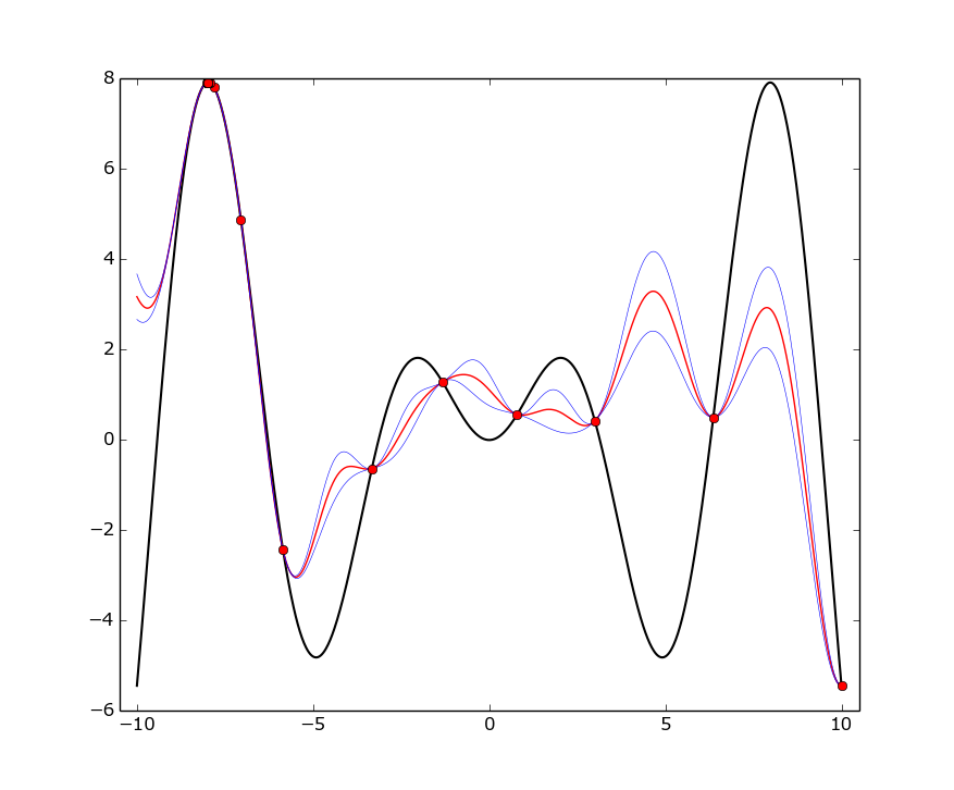
Example 1: the true function is 1-dimensional, f(x) = x * sin(x) (black curve) on [-10, 10] interval.
Red dots represent each trial, red curve is the Gaussian Process mean,
blue curve is the mean plus or minus one standard deviation.
The optimizer randomly chose the negative mode as more promising.
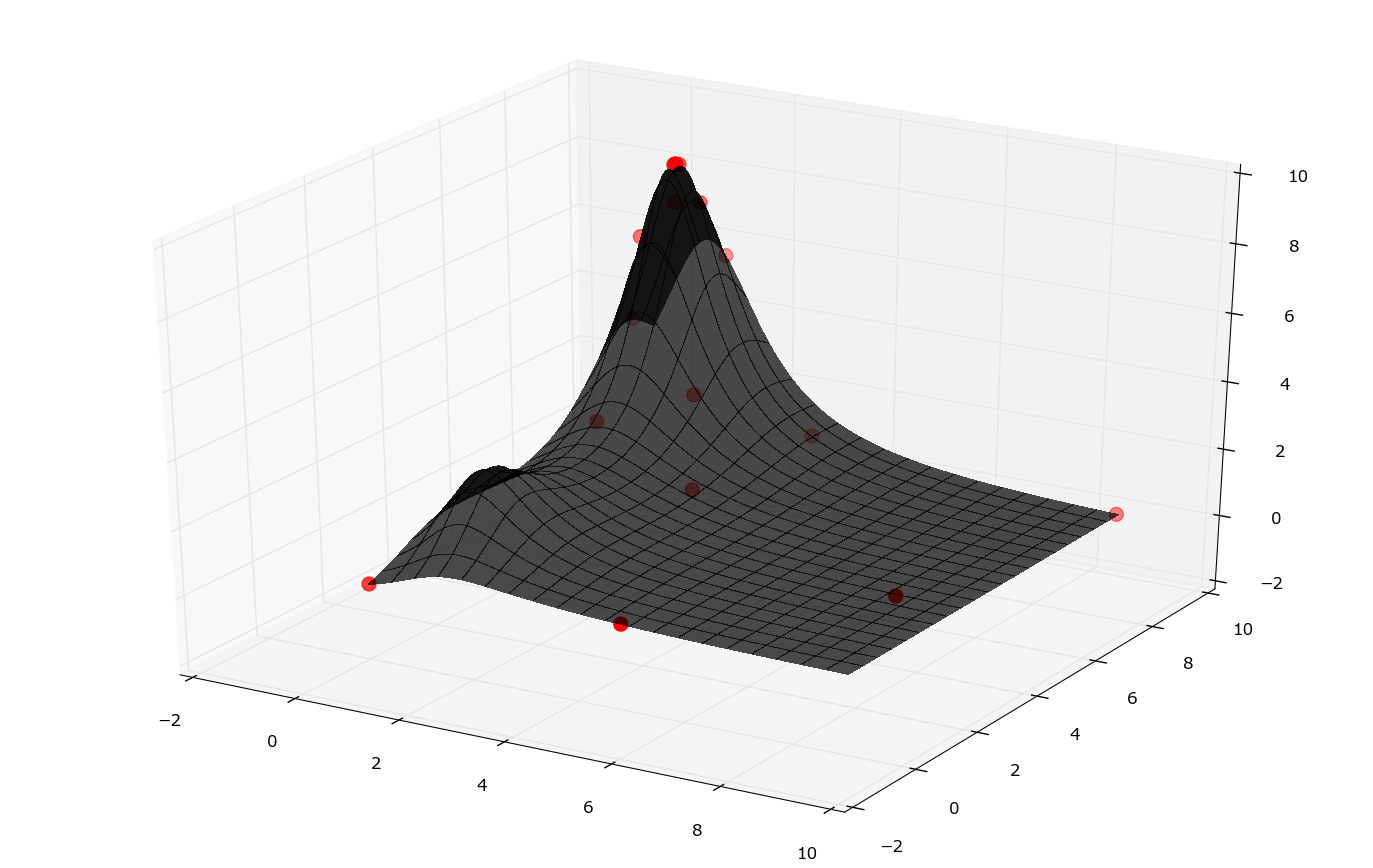
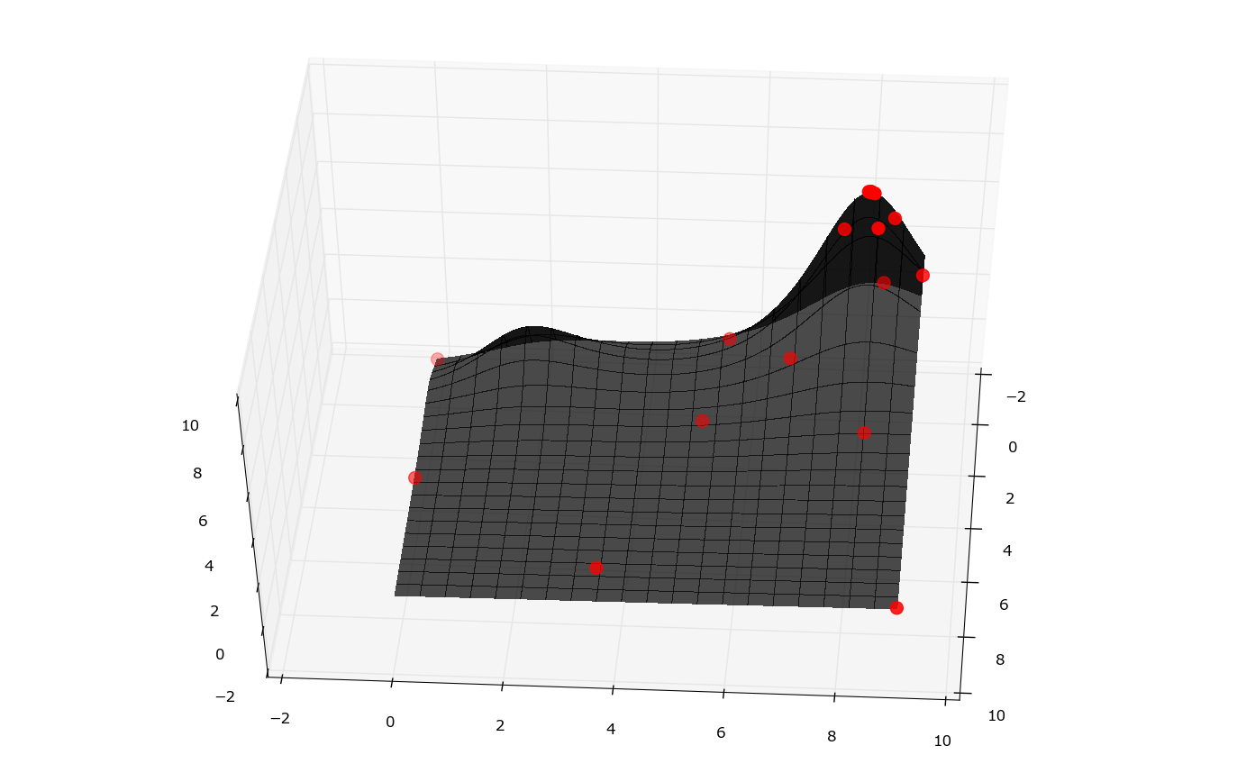
Example 2: the 2-dimensional function f(x, y) = (x + y) / ((x - 1) ** 2 - sin(y) + 2) (black surface) on [0,9]x[0,9] square.
Red dots represent each trial, the Gaussian Process mean and standard deviations are not shown for simplicity.
Note that to achieve the maximum both variables must be picked accurately.
The code for these and others examples is here.
HyperEngine can monitor the model performance during the training and stop early if it's learning too slowly. This is done via learning curve prediction. Note that this technique is compatible with Bayesian Optimization, since it estimates the model accuracy after full training - this value can be safely used to update Gaussian Process parameters.
Example code:
curve_params = {
  'burn_in': 30,                # burn-in period: 30 models
  'min_input_size': 5,          # start predicting after 5 epochs
  'value_limit': 0.80,          # stop if the estimate is less than 80% with high probability
}
curve_predictor = LinearCurvePredictor(**curve_params)
Currently there is only one implementation of the predictor, LinearCurvePredictor,
which is very efficient, but requires relatively large burn-in period to predict model accuracy without flaws.
Note that learning curves can be reused between different models and works quite well for the burn-in,
so it's recommended to serialize and load curve data via io_save_dir and io_load_dir parameters.
See also the following paper: Speeding up Automatic Hyperparameter Optimization of Deep Neural Networks by Extrapolation of Learning Curves
Implements the following methods:
- Probability of improvement (See H. J. Kushner. A new method of locating the maximum of an arbitrary multipeak curve in the presence of noise. J. Basic Engineering, 86:97–106, 1964.)
- Expected Improvement (See J. Mockus, V. Tiesis, and A. Zilinskas. Toward Global Optimization, volume 2, chapter The Application of Bayesian Methods for Seeking the Extremum, pages 117–128. Elsevier, 1978)
- Upper Confidence Bound
- Mixed / Portfolio strategy
- Naive random search.
PI method prefers exploitation to exploration, UCB is the opposite. One of the best strategies we've seen is a mixed one: start with high probability of UCB and gradually decrease it, increasing PI probability.
Default kernel function used is RBF kernel, but it is extensible.


