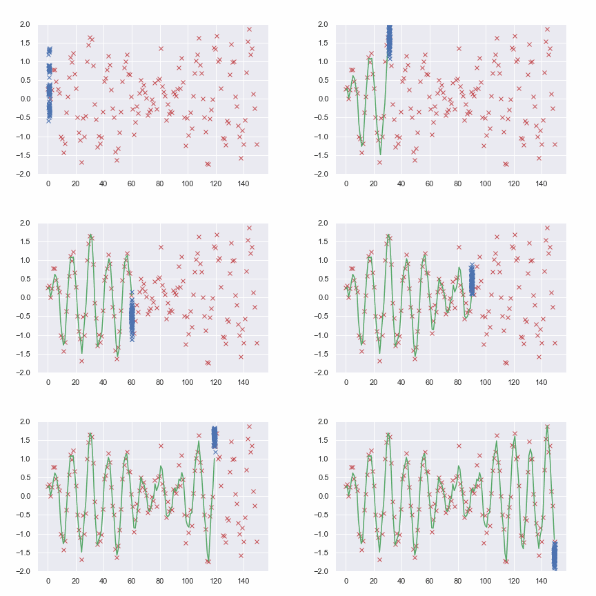
Contibutors:

FilterFlow (Beta)

A differentiable (and classical) TensorFlow implementation of Particle Filtering (SMC) techniques. If you are using this code in your research, please consider citing our paper.

@misc{dpf2021,
      title={Differentiable Particle Filtering via Entropy-Regularized Optimal Transport}, 
      author={Adrien Corenflos and James Thornton and Arnaud Doucet and George Deligiannidis},
      year={2021},
      eprint={2102.07850},
      archivePrefix={arXiv},
      primaryClass={stat.ML}
}

What is it?

Particle Filters (PF) [1] are a powerful class of methods for performing state inference in state-space models, and computing likelihood estimates for fixed parameters. Resampling is a key ingredient of PF, necessary to obtain low variance estimates. However, resampling operations result in the simulated likelihood function being non-differentiable with respect to parameters, even if the true likelihood is itself differentiable. This package leverages the ideas from Regularized Optimal Transport [2] to provide differentiable alternatives to these operations.

Supported features

Bootstrap Particle Filter
Custom Transition, Observation and Proposal Models
Gradient Backpropagation
Standard Resampling with biased gradients: Multinomial, Systematic, Stratified resampling
Differentiable Resampling: Differentiable Ensemble Transform (DET), Covariance Corrected DET, Variance Corrected DET, Optimized Point Cloud Resampling

Example

import matplotlib.pyplot as plt
import numpy as np
import tensorflow as tf
import tensorflow_probability as tfp

from filterflow import SMC, State, mean, std
from filterflow.observation import LinearObservationModel
from filterflow.proposal import BootstrapProposalModel
from filterflow.resampling import NeffCriterion, RegularisedTransform
from filterflow.transition import RandomWalkModel

tfd = tfp.distributions

# Generate artificial data.
rng = np.random.RandomState(42)
T = 150
noise = 0.5

# Here we simply use a noisy sine function
linspace = np.linspace(0., 5., T)
sine = np.sin(linspace)
noisy_sine = sine + np_random_state.normal(0., noise, T)
observations_dataset = tf.data.Dataset.from_tensor_slices(noisy_sine.astype(np.float32))

# Set the model.
sigma_x = 0.5
sigma_y = 1.
observation_matrix = tf.eye(1)
transition_matrix = tf.eye(1)

transition_noise = tfd.MultivariateNormalDiag(tf.constant([sigma_x]))
observation_error = tfd.MultivariateNormalDiag(0., tf.constant([sigma_y]))
transition_model = RandomWalkModel(transition_matrix, transition_noise)
observation_model = LinearObservationModel(observation_matrix, observation_error)
proposal_model = BootstrapProposalModel(transition_model)

# Let's resample when the ESS drops below 50%
resampling_criterion = NeffCriterion(0.5, is_relative=True)

# And use DET resampling
epsilon = tf.constant(0.5)
resampling_method = RegularisedTransform(epsilon)

# The SMC object
smc = SMC(observation_model, transition_model, proposal_model, resampling_criterion, resampling_method)

# The Initial state
batch_size = 5
n_particles = 50
dimension = 1
initial_particles = np_random_state.normal(0., 1., [batch_size, n_particles, dimension]).astype(np.float32)
initial_state = State(tf.convert_to_tensor(initial_particles))

# Run
state_series = smc(initial_state, observations_dataset, T, return_final=False, seed=555)

log_likelihoods = state_series.log_likelihoods
mean_particles = mean(state_series, keepdims=True)
std_particles = std(state_series, mean_particles) # the mean argument is optional

Installation

This project can be installed from its git repository.

Obtain the sources by:

git clone <https://github.com/repository>.git

or, if git is unavailable, download as a ZIP from GitHub https://github.com/.

Install:

python -m venv venv

source venv/bin/activate

pip install -r requirements.txt
Check examples:
- Simple tutorials are available in the notebooks folder.
- More comprehensive examples, used in our paper, are in the scripts folder.

References

.. [1] Arnaud Doucet, Nando de Freitas and Neil Gordon. Sequential Monte Carlo methods in practice. In: Springer Science & Business Media, 2001