The aim of darkest is to estimate dark adaptation biomarkers from raw dark adaptation data. The package darkest performs nonlinear curve fitting, along with validation and goodness-of-fit tests.
In contrast to previous R packages for dark adaptation data, darkest works perfectly with the tools of the tidyverse. This facilitates efficient fitting of multiple models across test-loci and patients, as well as bootstrapping. Importantly, bootstrapping enables the calculation of confidence intervals for derived parameters, that are not present in the initial fitting process (e.g., rod intercept time).
The package contains three types of functions:
-
Multistart wrapper functions for nonlinear dark adaptation curve fitting (currently, only a four parameter model of dark adapation is implemented; further models will be added)
multistart_fit_p4_model(data, start_value_grid) -
Function to select the best dark adaptation model among all fits based on the AIC
select_best_DA_fit(multistart_result) -
Bootstrap function to estimate the uncertainty of these curve fits
boot_DA_fit(data, start_value_grid, n)
Further, a function to extract derived parameters, that are not present in the initial fitting process (e.g., rod intercept time), and a dedicated plotting function will be added.
Maximilian Pfau, MD: maximilian.pfau@nih.gov
Brett Jeffrey, Ph.D.: brett.jeffrey@nih.gov
This is a basic example which shows you how to fit a four parameter dark
adaptation model with the functions multistart_fit_p4_model() and
select_best_DA_fit() :
library(darkest)

## Basic code

# Read example data, digitized from Fig. 6 in
# Jacobson SG. et al. IOVS. 2001 Jul;42(8):1882-90
data <- darkest::data

# Add pre-bleach data at 120 min to enhance model fit
data$Time <- ifelse(data$Time=="pre", 120, as.character(data$Time))
data$Time <- as.numeric(data$Time)


# Add noise (only for demonstration purposes,
# since bootstrap model fits will 'overlap'
# with the original data)
data$Threshold <- data$Threshold + rnorm(length(data$Threshold), 0, 0.25)


# Create grid with starting values
start_val_grid <- expand.grid(ct=seq(4.5,6.5,1),
                              CRbreak=seq(5,20,2),
                              S2=-0.24,
                              tf=1.5 )

# Define new data for curve plotting
new_df <- tibble::tibble(Time = seq(0, 70, 0.1))


# Fit dark adaptation models using the tools of the tidyverse
library(tidyverse)
#> Registered S3 method overwritten by 'rvest':
#>   method            from
#>   read_xml.response xml2
#> -- Attaching packages ---------------------------------- tidyverse 1.2.1 --
#> v ggplot2 3.3.2     v purrr   0.3.4
#> v tibble  3.0.4     v dplyr   1.0.2
#> v tidyr   1.1.2     v stringr 1.4.0
#> v readr   1.3.1     v forcats 0.5.0
#> Warning: package 'ggplot2' was built under R version 3.6.3
#> Warning: package 'tibble' was built under R version 3.6.3
#> Warning: package 'tidyr' was built under R version 3.6.3
#> Warning: package 'purrr' was built under R version 3.6.3
#> Warning: package 'dplyr' was built under R version 3.6.3
#> Warning: package 'forcats' was built under R version 3.6.3
#> -- Conflicts ------------------------------------- tidyverse_conflicts() --
#> x dplyr::filter() masks stats::filter()
#> x dplyr::lag()    masks stats::lag()

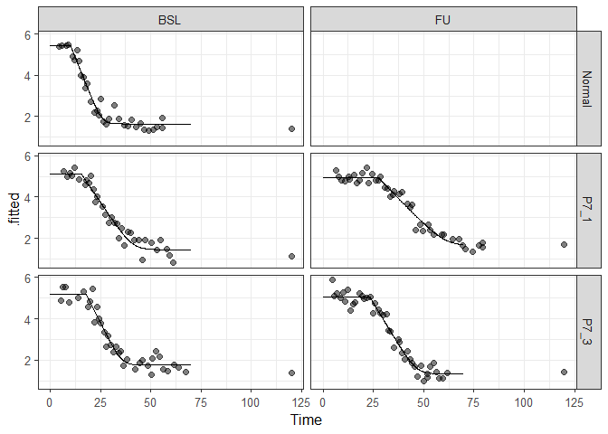
model_fits <- data %>%
  tidyr::nest(data=c("Time", "Threshold")) %>%
  dplyr::mutate(fit = purrr::map(data, ~ select_best_DA_fit(multistart_fit_p4_model(.x, start_val_grid))),
                augmented = purrr::map(fit, ~broom::augment(.x, newdata = new_df)) )

preds <- dplyr::select(model_fits, PID, VID, augmented) %>%
  tidyr::unnest(augmented)

ggplot2::ggplot() +
  geom_line(aes(Time, .fitted), preds) +
  geom_point(aes(Time, Threshold), data, size = 2, alpha = 0.5) +
theme_bw(base_size = 12) + facet_grid(PID ~ VID)This example shows how to bootstrap curve fits with the function
boot_DA_fit() to better understand the uncertainty of these curve fits
and their predictions.
## Basic code

boot_fits <- data %>%
  tidyr::nest(data=c("Time", "Threshold")) %>%
  dplyr::mutate(fit = purrr::map(data, ~ boot_DA_fit(.x, start_val_grid, 100)))

boot_preds <- boot_fits %>%
  tidyr::unnest(fit) %>% tidyr::unnest(boot_fits) %>%
  dplyr::mutate(id = dplyr::row_number()) %>%
  dplyr::mutate(augmented = purrr::map(fit, ~broom::augment(.x, newdata = new_df)) ) %>%
  tidyr::unnest(augmented)

ggplot2::ggplot() +
  geom_line(aes(Time, .fitted, group=id), boot_preds, alpha = 0.03, color="blue") +
  theme_bw(base_size = 12) + facet_grid(PID ~ VID) +
  geom_point(aes(Time, Threshold), data, size = 2, alpha = 0.5) +
  theme_bw(base_size = 12) + facet_grid(PID ~ VID) + xlim(0, 60)
#> Warning: Removed 50500 row(s) containing missing values (geom_path).
#> Warning: Removed 18 rows containing missing values (geom_point).

