Neural Flows: Efficient Alternative to Neural ODEs [arxiv]
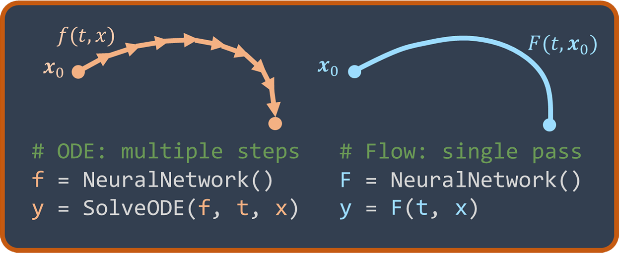
TL;DR: We directly model the neural ODE solutions with neural flows, which is much faster and achieves better results on time series applications, since it avoids using expensive numerical solvers.
Marin Biloš, Johanna Sommer, Syama Sundar Rangapuram, Tim Januschowski, Stephan Günnemann
Abstract: Neural ordinary differential equations describe how values change in time. This is the reason why they gained importance in modeling sequential data, especially when the observations are made at irregular intervals. In this paper we propose an alternative by directly modeling the solution curves - the flow of an ODE - with a neural network. This immediately eliminates the need for expensive numerical solvers while still maintaining the modeling capability of neural ODEs. We propose several flow architectures suitable for different applications by establishing precise conditions on when a function defines a valid flow. Apart from computational efficiency, we also provide empirical evidence of favorable generalization performance via applications in time series modeling, forecasting, and density estimation.
This repository acts as a supplementary material which implements the models and experiments as described in the main paper. The definition of models relies on the stribor package for normalizing and neural flows. The baselines use torchdiffeq package for differentiable ODE solvers.
Install the local package nfe (which will also install all the dependencies):
pip install -e .
Download and preprocess real-world data and generate synthetic data (or run commands in download_all.sh manually):
. scripts/download_all.sh
Many experiments will automatically download data if it's not already downloaded so this step is optional.
Note: MIMIC-III and IV have to be downloaded manually. Use notebooks in data_preproc to preprocess data.
After downloading everything, your directory tree should look like this:
├── nfe
│   ├── experiments
│   │   ├── base_experiment.py
│   │   ├── data
│   │   │   ├── activity
│   │   │   ├── hopper
│   │   │   ├── mimic3
│   │   │   ├── mimic4
│   │   │   ├── physionet
│   │   │   ├── stpp
│   │   │   ├── synth
│   │   │   └── tpp
│   │   ├── gru_ode_bayes
│   │   ├── latent_ode
│   │   ├── stpp
│   │   ├── synthetic
│   │   └── tpp
│   ├── models
│   └── train.py
├── scripts
│   ├── download_all.sh
│   └── run_all.sh
└── setup.py
Models are located in nfe/models. It contains the implementation of CouplingFlow and ResNetFlow. The ODE models and continuous (ODE or flow-based) GRU and LSTM layers can be found in the same directory.
import torch
from nfe import CouplingFlow

dim = 4
model = CouplingFlow(
    dim,
    n_layers=2, # Number of flow layers
    hidden_dims=[32, 32], # Hidden layers in single flow
    time_net='TimeLinear', # Time embedding network
)

t = torch.rand(3, 10, 1) # Time points at which IVP is evaluated
x0 = torch.randn(3, 1, dim) # Initial conditions at t=0

xt = model(x0, t) # IVP solutions at t given x0
xt.shape # torch.Size([3, 10, 4])import torch
from nfe import GRUFlow
dim = 4
model = GRUFlow(
dim,
n_layers=2, # Number of flow layers
hidden_dims=[32, 32], # Hidden layers in single flow
time_net='TimeTanh', # Time embedding network
)
t = torch.rand(3, 10, 1) # Time points at which IVP is evaluated
x = torch.randn(3, 10, dim) # Initial conditions, RNN inputs
xt = model(x, t) # IVP solutions at t_i given x_{1:i}
xt.shape # torch.Size([3, 10, 4])Run all experiments: . scripts/run_all.sh. Or run individual commands manually.
Example:
python -m nfe.train --experiment synthetic --data [ellipse|sawtooth|sink|square|triangle] --model [ode|flow] --flow-model [coupling|resnet] --solver [rk4|dopri5]
Example:
python -m nfe.train --experiment latent_ode --data [activity|hopper|physionet] --classify [0|1] --model [ode|flow] --flow-model [coupling|resnet]
Reference:
- Yulia Rubanova, Ricky Chen, David Duvenaud. "Latent ODEs for Irregularly-Sampled Time Series" (2019) [paper]. We adapted the code from here.
Request MIMIC-III and IV data, and download locally. Use notebooks to preprocess data.
Example:
python -m nfe.train --experiment gru_ode_bayes --data [mimic3|mimic4] --model [ode|flow] --odenet gru --flow-model [gru|resnet]
Reference:
- Edward De Brouwer, Jaak Simm, Adam Arany, Yves Moreau. "GRU-ODE-Bayes: Continuous modeling of sporadically-observed time series" (2019) [paper]. We adapted the code from here.
Example:
python -m nfe.train --experiment tpp --data [poisson|renewal|hawkes1|hawkes2|mooc|reddit|wiki] --model [rnn|ode|flow] --flow-model [coupling|resnet] --decoder [continuous|mixture] --rnn [gru|lstm] --marks [0|1]
Reference:
- Junteng Jia, Austin R. Benson. "Neural Jump Stochastic Differential Equations" (2019) [paper]. We adapted the code from here.
Example:
python -m nfe.train --experiment stpp --data [bike|covid|earthquake] --model [ode|flow] --density-model [independent|attention]
Reference:
- Ricky T. Q. Chen, Brandon Amos, Maximilian Nickel. "Neural Spatio-Temporal Point Processes" (2021) [paper]. We adapted the code from here.
@article{bilos2021neuralflows,
  title={{N}eural Flows: {E}fficient Alternative to Neural {ODE}s},
  author={Bilo{\v{s}}, Marin and Sommer, Johanna and Rangapuram, Syama Sundar and Januschowski, Tim and G{\"u}nnemann, Stephan},
  journal={Advances in Neural Information Processing Systems},
  year={2021}
}
