climateR seeks to simplifiy the steps needed to get climate data into
R. It currently provides access to the following gridded climate sources
using a single parmaeter
| Number | Dataset | Description | Dates |
|---|---|---|---|
| 1 | GridMET | Gridded Meteorological Data. | 1979 - Yesterday |
| 2 | Daymet | Daily Surface Weather and Climatological Summaries | 1980 - 2019 |
| 3 | TopoWX | Topoclimatic Daily Air Temperature Dataset | 1948 - 2016 |
| 4 | PRISM | Parameter-elevation Regressions on Independent Slopes | 1981 - (Yesterday-1) |
| 5 | MACA | Multivariate Adaptive Constructed Analogs | 1950 - 2099 |
| 6 | LOCA | Localized Constructed Analogs | 1950 - 2100 |
| 7 | BCCA | Bias Corrected Constructed Analogs | 1950 - 2100 |
| 8 | BCSD | Bias Corrected Spatially Downscaled VIC: Monthly Hydrology | 1950 - 2099 |
| 9 | TerraClimate | TerraClimate Monthly Gridded Data | 1958 - 2019 |
| 10 | CHIRPS | Climate Hazards Group InfraRed Precipitation with Station | 1980 - Current month |
| 11 | EDDI | Evaporative Demand Drought Index | 1980 - Current year |
remotes::install_github("mikejohnson51/AOI") # suggested!
remotes::install_github("mikejohnson51/climateR")library(AOI)
library(climateR)
library(sf)
library(raster)
library(rasterVis)The climateR package is supplimented by the AOI framework established in the AOI R package.
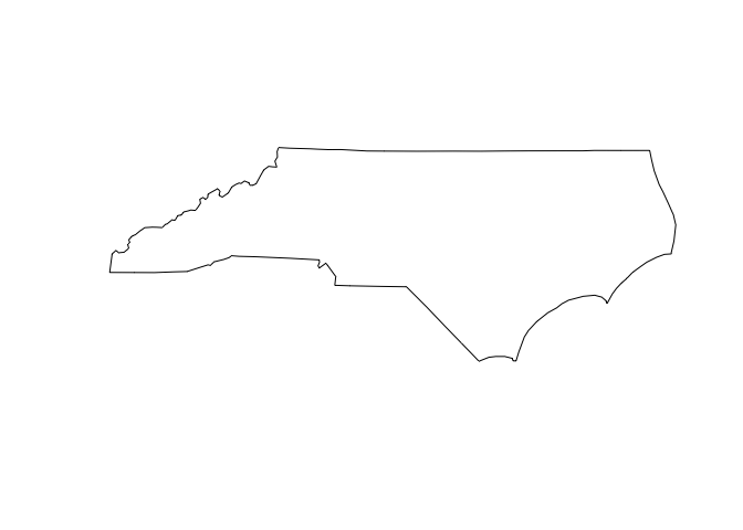
To get a climate product, an area of interest must be defined:
AOI = aoi_get(state = "NC")
plot(AOI$geometry)
Here we are loading a polygon for the state of California. More examples of constructing AOI calls can be found here.
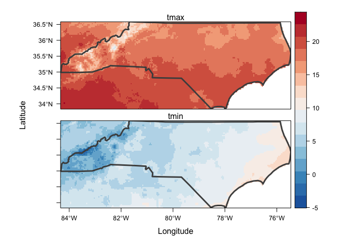
With an AOI, we can construct a call to a dataset for a parameter(s) and date(s) of choice. Here we are querying the PRSIM dataset for maximum and minimum temperature on October 29, 2018:
system.time({
 p = getPRISM(AOI, param = c('tmax','tmin'), startDate = "2018-10-29")
})
#>    user  system elapsed
#>   0.933   0.376   6.808
r = raster::stack(p)
names(r) = names(p)
rasterVis::levelplot(r, par.settings = BuRdTheme) +
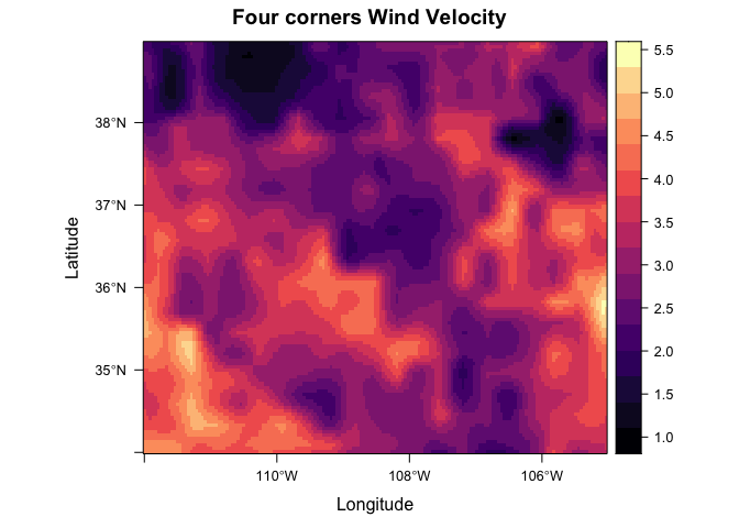
layer(sp.lines(as_Spatial(AOI), col="gray30", lwd=3))climateR offers support for sf, sfc, and bbox objects. Here we
are requesting wind velocity data for the four corners region of the USA
by bounding coordinates.
AOI = st_bbox(c(xmin = -112, xmax = -105, ymax = 39, ymin = 34), crs = 4326) %>%
  getGridMET(param = "wind_vel", startDate = "2018-09-01")

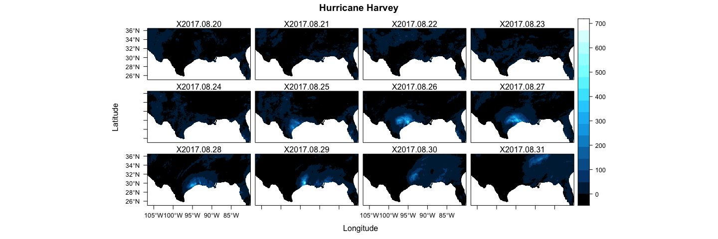
rasterVis::levelplot(AOI$wind_vel, margin = FALSE, main = "Four corners Wind Velocity")In addition to multiple variables we can request variables through time, here let’s look at the gridMET rainfall for the Gulf Coast during Hurricane Harvey:
harvey = getGridMET(aoi_get(state = c("TX", "FL")),
                  param = "prcp",
                  startDate = "2017-08-20", endDate = "2017-08-31")

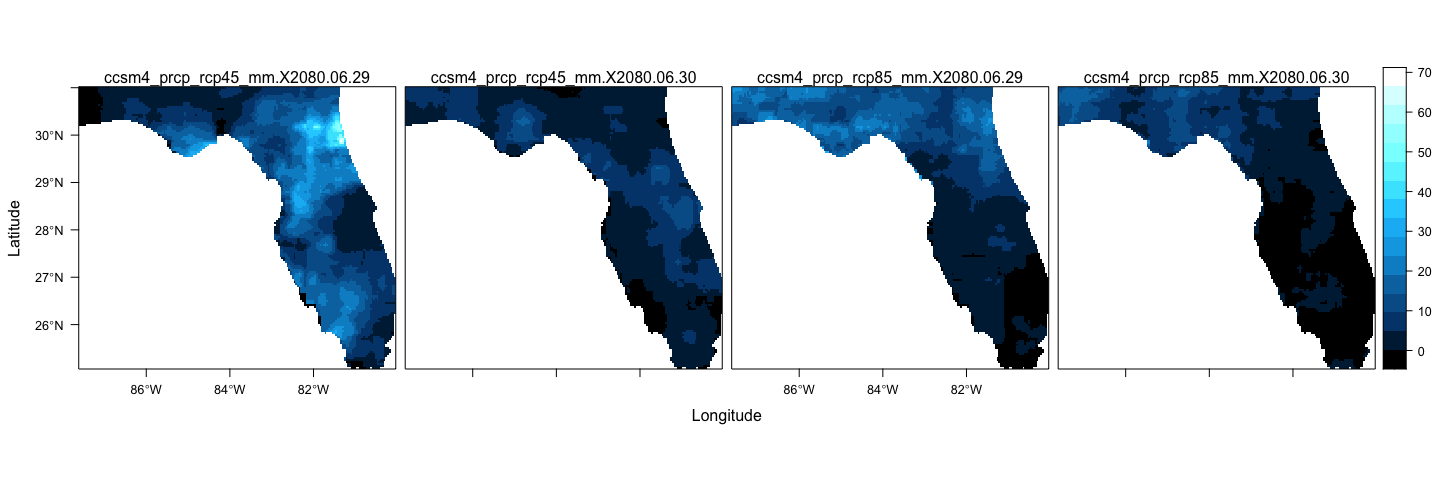
levelplot(harvey$prcp, par.settings = BTCTheme, main = "Hurricane Harvey")Some sources are downscaled Global Climate Models (GCMs). These allow you to query forecasted ensemble members from different models and/or climate scenarios. One example is from the MACA dataset:
system.time({
m = getMACA(aoi_get(state = "FL"),
            model = "CCSM4",
            param = 'prcp',
            scenario = c('rcp45', 'rcp85'),
            startDate = "2080-06-29", endDate = "2080-06-30")
})
#>    user  system elapsed
#>   0.346   0.137   4.235
r = raster::stack(m)
names(r) = paste(rep(names(m), each = 2), names(m[[1]]))
levelplot(r, par.settings = BTCTheme)Getting multiple models results is also quite simple:
models = c("bnu-esm","canesm2", "ccsm4", "cnrm-cm5", "csiro-mk3-6-0")
temp = getMACA(AOI = aoi_get(state = "conus"),
param = 'tmin',
model = models,
startDate = "2080-11-29")
s = stack(temp)
s = addLayer(s, mean(s))
names(s) = c(models, "Ensemble Mean")
# Plot
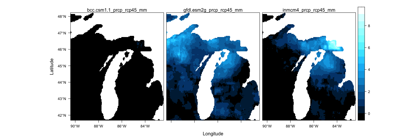
rasterVis::levelplot(s, par.settings = rasterVis::BuRdTheme)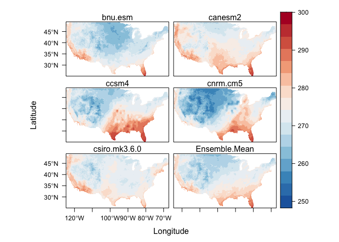 If
you don’t know your models, you can always grab a random set by
specifying a number:
random = getMACA(aoi_get(state = "MI"), model = 3, param = "prcp", startDate = "2050-10-29")
random = stack(random) %>% setNames(names(random))
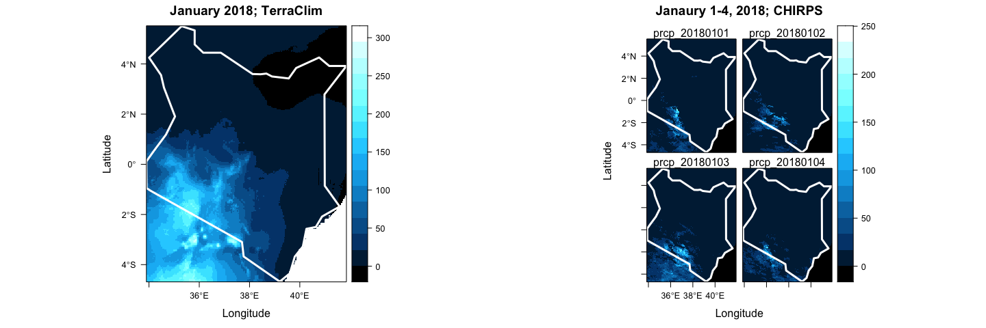
levelplot(stack(random), par.settings = BTCTheme)Not all datasets are USA focused either. TerraClimate offers global, monthly data up to the current year for many variables, and CHIRPS provides daily rainfall data:
kenya = aoi_get(country = "Kenya")
tc = getTerraClim(kenya, param = "prcp", startDate = "2018-01-01")
chirps = getCHIRPS(kenya, startDate = "2018-01-01", endDate = "2018-01-04" )

p1 = levelplot(tc$prcp, par.settings = BTCTheme, main = "January 2018; TerraClim", margin = FALSE) +
  layer(sp.lines(as_Spatial(kenya), col="white", lwd=3))
p2 = levelplot(chirps,  par.settings = BTCTheme, main = "Janaury 1-4, 2018; CHIRPS", layout=c(2, 2)) +
  layer(sp.lines(as_Spatial(kenya), col="white", lwd=3))

gridExtra::grid.arrange(p1,p2, nrow = 1)
This raises the question “what is available for each resource?”. This
can be checked in the appropriate meta_data objects. For example let’s
see what parameter data is offered for gridMET, and what models and
scenarios are offered for MACA.
head(param_meta$gridmet)
#>   common.name call                               description
#> 1        prcp   pr                      precipitation_amount
#> 2       rhmax rmax           daily_maximum_relative_humidity
#> 3       rhmin rmin           daily_minimum_relative_humidity
#> 4        shum  sph              daily_mean_specific_humidity
#> 5        srad srad daily_mean_shortwave_radiation_at_surface
#> 6    wind_dir   th                 daily_mean_wind_direction
#>                          units
#> 1                           mm
#> 2                      Percent
#> 3                      Percent
#> 4                        kg/kg
#> 5                        W/m^2
#> 6 Degrees Clockwise from north

head(model_meta$maca)
#>           model ensemble scenario
#> 1       BNU-ESM   r1i1p1    rcp45
#> 2      CNRM-CM5   r1i1p1    rcp45
#> 3 CSIRO-Mk3-6-0   r1i1p1    rcp45
#> 4    bcc-csm1-1   r1i1p1    rcp45
#> 5       CanESM2   r1i1p1    rcp45
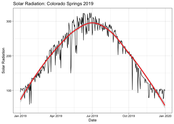
#> 6 GFDL-ESM2G r1i1p1 rcp45Finally, data gathering is not limited to areal extents and can be retrieved as a time series at locations.
AOI = AOI::geocode('Colorado Springs', pt = TRUE)
ts  = getGridMET(AOI, param = 'srad', startDate = "2019-01-01", endDate = "2019-12-31")

ggplot(data = ts) +
  aes(x = date, y = srad) +
  geom_line() +
  stat_smooth(col = "red") +
  theme_linedraw() +
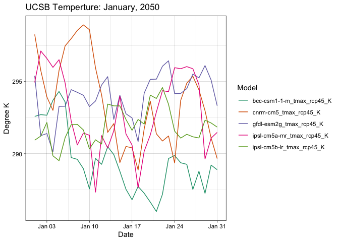
labs(title = "Solar Radiation: Colorado Springs 2019", x = "Date", y = "Solar Radiation")future = getMACA(geocode("UCSB", pt = TRUE),
model = 5, param = "tmax",
startDate = "2050-01-01", endDate = "2050-01-31")
future_long = future %>%
dplyr::select(-source, -lat, -lon) %>%
tidyr::pivot_longer(-date)
ggplot(data = future_long, aes(x = date, y = value, col = name)) +
geom_line() +
theme_linedraw() +
scale_color_brewer(palette = "Dark2") +
labs(title = "UCSB Temperture: January, 2050",
x = "Date",
y = "Degree K",
color = "Model")Extracting data for a set of points is an interesting challenge. It turns it is much more efficient to grab the underlying raster stack and then extract timeseries as opposed to iterating over the locations:
- Starting with a set of locations in Brazil:
(sites = read.csv('./inst/extdata/example.csv') %>%
  st_as_sf(coords = c("long", "lat"), crs = 4326))
#> Simple feature collection with 100 features and 2 fields
#> geometry type:  POINT
#> dimension:      XY
#> bbox:           xmin: -54.81975 ymin: -29.73627 xmax: -40.80975 ymax: -18.52627
#> geographic CRS: WGS 84
#> First 10 features:
#>         X     ID                    geometry
#> 1  190760 190760 POINT (-50.40975 -25.81627)
#> 2  267801 267801 POINT (-48.15975 -24.60627)
#> 3  219885 219885 POINT (-49.28975 -25.32627)
#> 4  200445 200445 POINT (-50.45975 -25.63627)
#> 5   74789  74789 POINT (-51.70975 -28.01627)
#> 6   18343  18343 POINT (-50.35975 -29.33627)
#> 7  143615 143615 POINT (-49.33975 -26.73627)
#> 8  588292 588292 POINT (-47.57975 -21.27627)
#> 9  371314 371314 POINT (-47.76975 -23.28627)
#> 10 638894 638894 POINT (-46.99975 -20.75627)climateRwill grab the RasterStack underlying the bounding area of the points
sites_stack = getTerraClim(AOI = sites,
                           param ="tmax",
                           startDate = "2018-01-01", endDate = "2018-12-31")


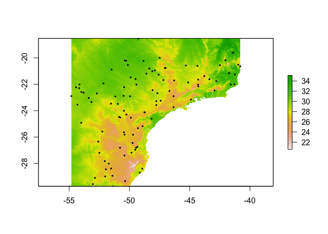
plot(sites_stack$tmax$X2018.01)
plot(sites$geometry, add = TRUE, pch = 16, cex = .5)- Use
extract_sitesto extract the times series from these locations. Theidparameter is the unique identifier from the site data with which to names the resulting columns.
sites_wide = extract_sites(sites_stack, sites, "ID")
sites_wide$tmax[1:5, 1:5]
#>         date site_190760 site_267801 site_219885 site_200445
#> 1 2018-01-01        26.9        31.5        25.6        26.2
#> 2 2018-02-01        26.6        30.1        25.2        25.8
#> 3 2018-03-01        26.4        30.8        25.6        26.0
#> 4 2018-04-01        25.3        28.3        24.8        24.9
#> 5 2018-05-01        21.5        25.1        21.7        21.2
To make the data ‘tidy’ simply pivot on the date column:
tmax = tidyr::pivot_longer(sites_wide$tmax, -date)
head(tmax)
#> # A tibble: 6 x 3
#>   date       name        value
#>   <date>     <chr>       <dbl>
#> 1 2018-01-01 site_190760  26.9
#> 2 2018-01-01 site_267801  31.5
#> 3 2018-01-01 site_219885  25.6
#> 4 2018-01-01 site_200445  26.2
#> 5 2018-01-01 site_74789   26.7
#> 6 2018-01-01 site_18343   24

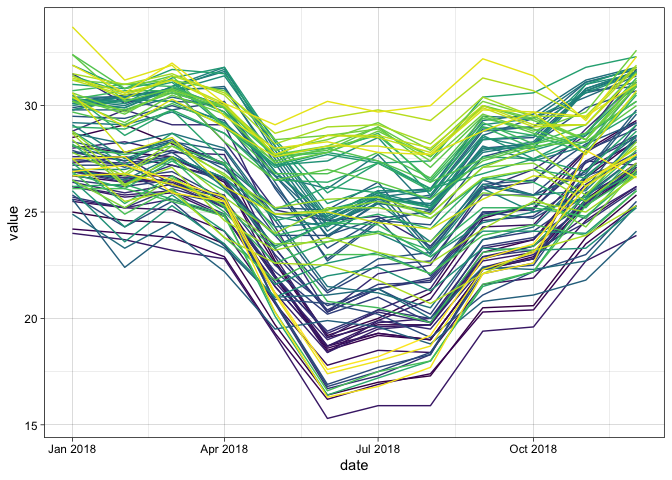
ggplot(data = tmax, aes(x = date, y = value, col = name)) +
  scale_color_viridis_d() +
  geom_line() +
  theme_linedraw() +
theme(legend.position = "none") ClimateR is written by Mike Johnson, a graduate Student at the University of California, Santa Barbara in Keith C. Clarke’s Lab.
