The HonestDiD package implements the tools for robust inference and sensitivity analysis for differences-in-differences and event study designs developed in Rambachan and Roth (2022). This is the Stata version of the R package of the same name. There is also a Shiny app developed by Chengcheng Fang.
version 1.3.1 16Apr2024 | Background | Installation | Examples | Acknowledgements
The robust inference approach in Rambachan and Roth formalizes the intuition that pre-trends are informative about violations of parallel trends. They provide a few different ways of formalizing what this means.
Bounds on relative magnitudes. One way of formalizing this idea is
to say that the violations of parallel trends in the post-treatment
period cannot be much bigger than those in the pre-treatment period.
This can be formalized by imposing that the post-treatment violation of
parallel trends is no more than some constant
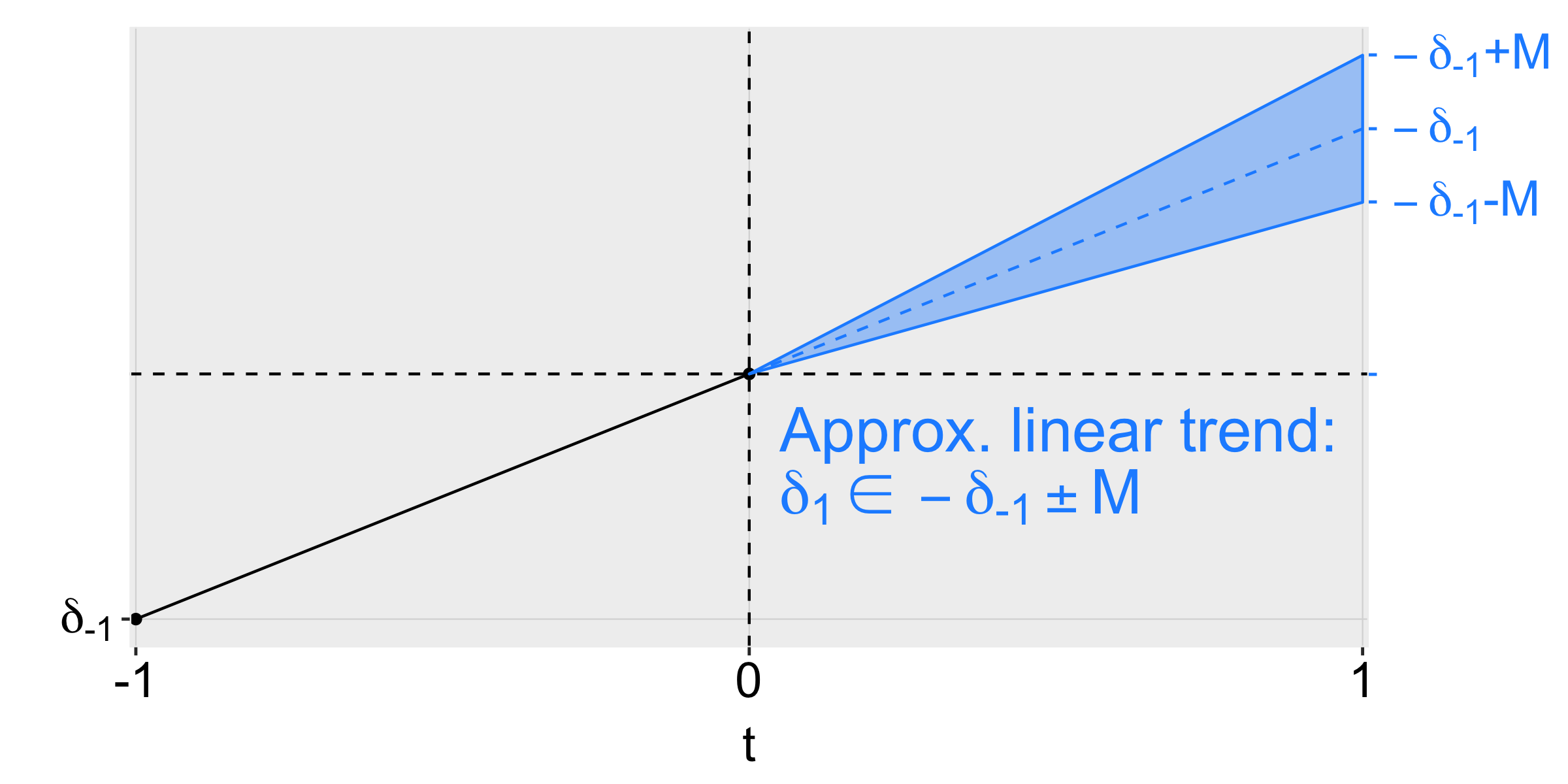
Smoothness restrictions. A second way of formalizing this is to say that the post-treatment violations of parallel trends cannot deviate too much from a linear extrapolation of the pre-trend. In particular, we can impose that the slope of the pre-trend can change by no more than M across consecutive periods, as shown in the figure below for an example with three periods.
Thus, imposing a smoothness restriction with
Other restrictions. The Rambachan and Roth framework allows for a variety of other restrictions on the differences in trends as well. However, not all these have yet been implemented in this Stata version of the package. This functionality is planned for a future release.
Robust confidence intervals. Given restrictions of the type described above, Rambachan and Roth provide methods for creating robust confidence intervals that are guaranteed to include the true parameter at least 95% of the time when the imposed restrictions on satisfied. These confidence intervals account for the fact that there is estimation error both in the treatment effects estimates and our estimates of the pre-trends.
Sensitivity analysis. The approach described above naturally lends
itself to sensitivity analysis. That is, the researcher can report
confidence intervals under different assumptions about how bad the
post-treatment violation of parallel trends can be (e.g., different
values of
The package may be installed by using net install for the latest version:
local github https://raw.githubusercontent.com
net install honestdid, from(`github'/mcaceresb/stata-honestdid/main) replace
honestdid _plugin_check
Version 1.3.0 (25Jan2024) of the package is currently available via SSC:
ssc install honestdid
honestdid _plugin_checkhonestdid uses compiled C code internally; if you receive an error
message saying "Failed to load OSQP/ECOS plugin" then you will need
to compile the plugin in order to use honestdid. While we provide
pre-compiled binaries, they may not work on every system. If you are
using OSX or Linux, compiling is relatively straightforward. From a
terminal, run:
git clone https://github.com/mcaceresb/stata-honestdid
cd stata-honestdid
bash src/compile.sh
You're required to have make, cmake, and clang (OSX) or gcc
(Linux) installed; all three should be readily available on any OSX or
Linux system. On Windows:
- Install Cygwin.
- Install
binutils,make,cmake,gcc-core,gcc-g++,mingw64-x86_64-gcc-core,mingw64-x86_64-gcc-g++,mingw64-x86_64-dlfcn - Open the Cygwin terminal and run
git clone https://github.com/mcaceresb/stata-honestdid
cd stata-honestdid
sed -i 's/\r$//' src/compile.sh
bash src/compile.sh
Once the plugin is compiled, from a Stata session run
cd /path/to/stata-honestdid/
do src/install.do
(On Windows, the repo will likely be somewhere in C:\cygwin64\home\..,
depending on where you installed Cygwin.) If compiling the plugin yourself does
not fix it, please open an issue.
As an illustration of the package, we will examine the effects of Medicaid expansions on insurance coverage using publicly-available data derived from the ACS. We first load the data and packages relevant for the analysis.
* Install here coefplot, ftools, reghdfe, plot scheme
local github https://raw.githubusercontent.com
ssc install coefplot,      replace
ssc install ftools,        replace
ssc install reghdfe,       replace
net install scheme-modern, replace from(`github'/mdroste/stata-scheme-modern/master)
set scheme modern

* Load data
local mixtape https://raw.githubusercontent.com/Mixtape-Sessions
use `mixtape'/Advanced-DID/main/Exercises/Data/ehec_data.dta, clear
l in 1/5
+--------------------------------------------+
| stfips year dins yexp2 W |
|--------------------------------------------|
1. | alabama 2008 .6814122 . 613156 |
2. | alabama 2009 .6580621 . 613156 |
3. | alabama 2010 .6313651 . 613156 |
4. | alabama 2011 .6563886 . 613156 |
5. | alabama 2012 .6708115 . 613156 |
+--------------------------------------------+
The data is a state-level panel with information on health insurance
coverage and Medicaid expansion. The variable dins shows the share of
low-income childless adults with health insurance in the state. The
variable yexp2 gives the year that a state expanded Medicaid coverage
under the Affordable Care Act, and is missing if the state never
expanded.
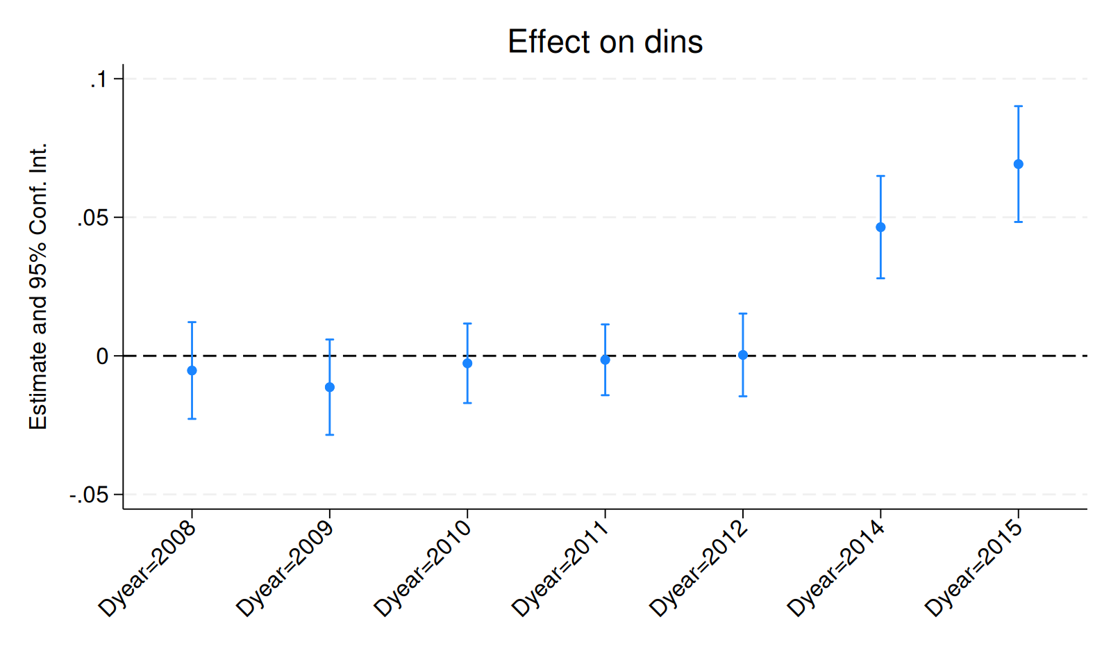
For simplicity, we will first focus on assessing sensitivity to violations of parallel trends in a non-staggered DiD (see below regarding methods for staggered timing). We therefore restrict the sample to the years 2015 and earlier, and drop the small number of states who are first treated in 2015. We are now left with a panel dataset where some units are first treated in 2014 and the remaining units are not treated during the sample period. We can then estimate the effects of Medicaid expansion using a canonical two-way fixed effects event-study specification,
where
* Keep years before 2016. Drop the 2016 cohort
keep if (year < 2016) & (missing(yexp2) | (yexp2 != 2015))

* Create a treatment dummy
gen byte D = (yexp2 == 2014)
gen `:type year' Dyear = cond(D, year, 2013)

* Run the TWFE spec
reghdfe dins b2013.Dyear, absorb(stfips year) cluster(stfips) noconstant

local plotopts ytitle("Estimate and 95% Conf. Int.") title("Effect on dins")
coefplot, vertical yline(0) ciopts(recast(rcap)) xlabel(,angle(45)) `plotopts'We are now ready to apply the HonestDiD package to do sensitivity
analysis. Suppose we’re interested in assessing the sensitivity of
the estimate for 2014, the first year after treatment. The pre() and
post() options specify the indices of the coefficients corresponding
with pre-treatment and post-treatment event-study coefficients
(excluding the one for 2013, which is normalized to zero); Stata's
numlist notation is allowed. Finally, mvec() specifies the values of
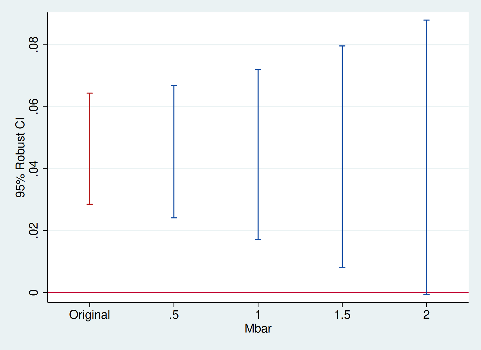
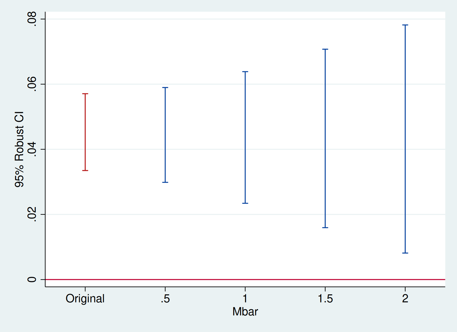
honestdid, pre(1/5) post(7/8) mvec(0.5(0.5)2)| M | lb | ub |
| ------- | ------ | ------ |
| . | 0.029 | 0.064 | (Original)
| 0.5000 | 0.024 | 0.067 |
| 1.0000 | 0.017 | 0.072 |
| 1.5000 | 0.008 | 0.080 |
| 2.0000 | -0.001 | 0.088 |
(method = C-LF, Delta = DeltaRM, alpha = 0.050)
First, note in this case the coefficients are ordered and mostly
contiguous, so pre(1/5) refers to entries 1 through 5 and post(7/8)
refers to entries 7 through 8. If the coefficients happen to be in
different orders, positions, or if there are controls included in the
regression, the user can pass an arbitrary list of indices to pre()
and post(). For instance,
honestdid, pre(1 2 3 4 5) post(7 8) mvec(0.5(0.5)2)gives the same result. Second, note the coefficient vector returned by
reghdfe includes an entry for 2013, the reference period, which was
omitted from the regression but is included in the vector of estimates.
It is possible to tell honestdid to ignore omitted regressors when
specifying variable indices; this can be specially useful when there
are many such covariates. For example,
reghdfe dins b2013.year##D, absorb(stfips year) cluster(stfips) noconstant
matrix list e(b)
honestdid, pre(1/5) post(6/7) mvec(0.5(0.5)2) omit
gives the same results (i.e. the coefficient vector contains several
zeros from omitted regressors, but with the omit option we only needed
to specify the indices for the included regressors). It's important that
here the post-period indices are 6 and 7, since the reference period is
no longer included. Further, the omit option does not exclude
zeros; rather, it excludes vector entries indicated to have been omitted
from a regression (based on the column names of the coefficient vector;
see help _ms_omit_info for more).
Finally, in the special case where there are no controls or where the
user has gathered the pre- and post-treatment coefficients into a custom
vector, it is also possible to specify just the number of pre-treatment
periods via numpre() and honestdid will automatically assume the
first numpre entries are pre-treatment coefficients and the rest are
post-treatment coefficients.
reghdfe dins b2013.Dyear, absorb(stfips year) cluster(stfips) noconstant
honestdid, numpre(5) mvec(0.5(0.5)2) omit

mata index = 1..5, 7..8
mata st_matrix("b", st_matrix("e(b)")[index])
mata st_matrix("V", st_matrix("e(V)")[index, index])
matrix list b
matrix list V
honestdid, numpre(5) mvec(0.5(0.5)2)
In all cases, the output of the honestdid command shows a robust
confidence interval for different values of
We can also visualize the sensitivity analysis using the coefplot
option. We can pass the option at the time of the CI computation or we
can use the last results from honestdid (which are cached in memory).
honestdid, coefplot cachedAdditional options are passed to coefplot
local plotopts xtitle(Mbar) ytitle(95% Robust CI)
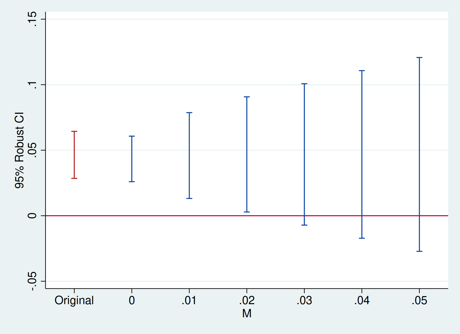
honestdid, cached coefplot `plotopts'We can also do a sensitivity analysis based on smoothness
restrictions---i.e. imposing that the slope of the difference in trends
changes by no more than
local plotopts xtitle(M) ytitle(95% Robust CI)
honestdid, pre(1/5) post(6/7) mvec(0(0.01)0.05) delta(sd) omit coefplot `plotopts'
| M | lb | ub |
| ------- | ------ | ------ |
| . | 0.029 | 0.064 | (Original)
| 0.0000 | 0.026 | 0.061 |
| 0.0100 | 0.013 | 0.079 |
| 0.0200 | 0.003 | 0.091 |
| 0.0300 | -0.007 | 0.101 |
| 0.0400 | -0.017 | 0.111 |
| 0.0500 | -0.027 | 0.121 |
(method = FLCI, Delta = DeltaSD, alpha = 0.050)
We see that the breakdown value for a significant effect is
So far we have focused on the effect for the first post-treatment
period, which is the default in HonestDiD. If we are instead interested
in the average over the two post-treatment periods, we can use the
option l_vec(matrix_name):
matrix l_vec = 0.5 \ 0.5
local plotopts xtitle(Mbar) ytitle(95% Robust CI)
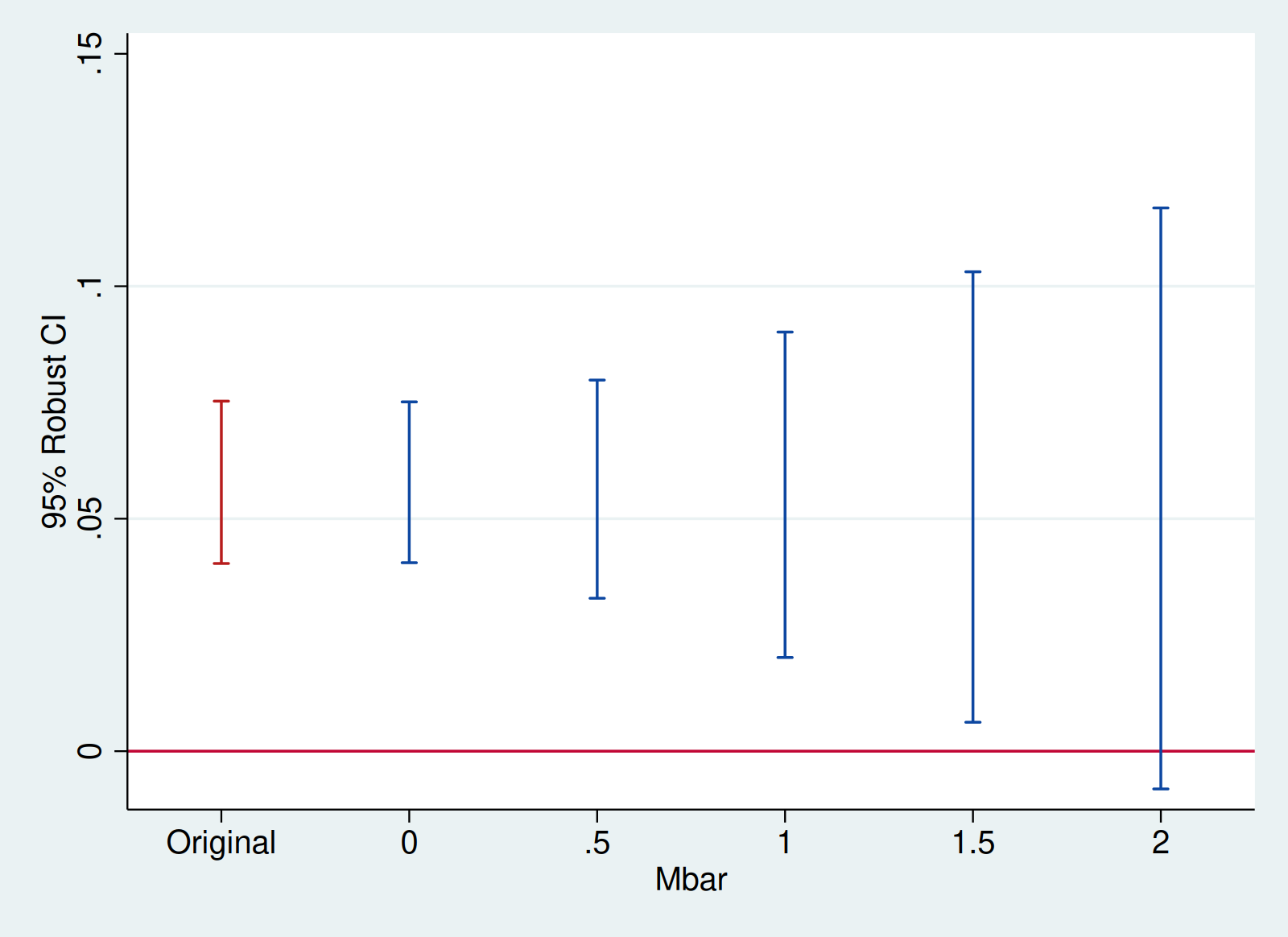
honestdid, l_vec(l_vec) pre(1/5) post(6/7) mvec(0(0.5)2) omit coefplot `plotopts'
|    M    |   lb   |   ub   |
| ------- | ------ | ------ |
|       . |  0.040 |  0.075 | (Original)
|  0.0000 |  0.041 |  0.075 |
|  0.5000 |  0.033 |  0.080 |
|  1.0000 |  0.020 |  0.090 |
|  1.5000 |  0.006 |  0.103 |
|  2.0000 | -0.008 |  0.117 |
(method = C-LF, Delta = DeltaRM, alpha = 0.050)
More generally, the package accommodates inference on any scalar
parameter of the form matrix l_vec = 0 \ 1
and setting l_vec(l_vec) allows us to do inference on the effect for
the second period after treatment.
honestdid has built-in support for the user-written
parallel package (latest stable
version required). parallel(#) can be specified as an option with #
signifying the number of cores (parallel processes; default 4). Each
core processes an
net install parallel, from(https://raw.github.com/gvegayon/parallel/stable) replace
mata mata mlib index
honestdid, pre(1/5) post(7/8) mvec(0.5(0.5)2) parallel(4)
processes each entry of mvec in a different core (with 8 values, 2
would be processed per core and so on; further, if more cores than parallel
package creates several temporary files in the current working directory;
honestdid runs parallel clean to delete them after a successful
run, but in case of an error the user may need to delete them manually.
So far we have focused on a simple case without staggered timing. Fortunately, the HonestDiD approach works well with recently-introduced methods for DiD under staggered treatment timing. Below, we show how the package can be used with the did package implementing Callaway and Sant’Anna. We are hoping to more formally integrate the did and HonestDiD packages in the future---stay tuned!
local mixtape https://raw.githubusercontent.com/Mixtape-Sessions
use `mixtape'/Advanced-DID/main/Exercises/Data/ehec_data.dta, clear
qui sum year, meanonly
replace yexp2 = cond(mi(yexp2), r(max) + 1, yexp2)
qui csdid dins, time(year) ivar(stfips) gvar(yexp2) long2 notyet
csdid_estat event, window(-4 5) estore(csdid)
estimates restore csdid

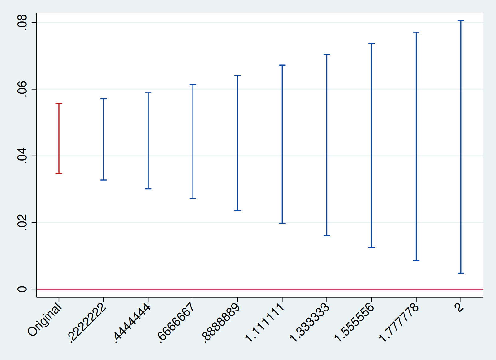
local plotopts xtitle(Mbar) ytitle(95% Robust CI)
honestdid, pre(3/6) post(7/12) mvec(0.5(0.5)2) coefplot `plotopts'HonestDiD is also compatible with the estimator introduced in
Chaisemartin and D'Haultfoeuille (2020), available for Stata
via the did_multiplegt package.
local mixtape https://raw.githubusercontent.com/Mixtape-Sessions
use `mixtape'/Advanced-DID/main/Exercises/Data/ehec_data.dta, clear
gen byte D = (year >= yexp2) & !mi(yexp2)
did_multiplegt dins stfips year D, robust_dynamic dynamic(5) placebo(5) breps(50) cluster(stfips)
honestdid, pre(7/11) post(1/6) vcov(didmgt_vcov) b(didmgt_results_no_avg)You can view a video presentation about this paper here.
This software package is based upon work supported by the National Science Foundation Graduate Research Fellowship under Grant DGE1745303 (Rambachan) and Grant DGE1144152 (Roth).
