For a complete description of how the project runs, clone the repo and view Traffic_Sign_Classifier.html.
The goals / steps are the following:
- Load the data set (see below for links to the project data set)
- Explore, summarize and visualize the data set
- Design, train and test a model architecture
- Use the model to make predictions on new images
- Analyze the softmax probabilities of the new images
- Summarize the results with a written report
My project code is included in this repository (Traffic_Sign_Classifier.ipynb). An html file containing the code along with output for a complete run is also included (Traffic_Sign_Classifier.html).
Unfortunately the training/validation/test datasets were too big to upload. You can run this notebook, but only if you clone the repo and add the "traffic-signs-data" directory containing "test.p," "train.p," and "valid.p."
I installed TensorFlow with GPU support on my laptop, which has an Nvidia GPU.
TensorFlow with GPU support was observed to train my network
roughly 9X faster than the CPU-only version.
Without GPU support, the lab would have been infeasibly time-consuming.
My project code is included in this repository (Traffic_Sign_Classifier.ipynb). An html file containing the code along with output for a complete run is also included (Traffic_Sign_Classifier.html).
1. Provide a basic summary of the data set. In the code, the analysis should be done using python, numpy and/or pandas methods rather than hardcoding results manually.
I used the len() function to determine size of training, validation, and test sets, and the shape attribute to determine individual image shape.
- The size of training set is 34799.
- The size of the validation set is 4410.
- The size of test set is 12630.
- The shape of a traffic sign image is 32x32x3.
- The number of unique classes/labels in the data set is 43.
Please refer to heading Include an exploration visualization of the dataset in the html output. A sample image from the training set is shown along with its label. Also, a histogram of the number of images of each type in each set is shown for all three sets. Some sign types are underrepresented, although the distribution of sign types in the training, validation, and test sets is surprisingly similar.
1. Describe how you preprocessed the image data. What techniques were chosen and why did you choose these techniques? Consider including images showing the output of each preprocessing technique. Pre-processing refers to techniques such as converting to grayscale, normalization, etc. (OPTIONAL: As described in the "Stand Out Suggestions" part of the rubric, if you generated additional data for training, describe why you decided to generate additional data, how you generated the data, and provide example images of the additional data. Then describe the characteristics of the augmented training set like number of images in the set, number of images for each class, etc.)
I did not consider converting to grayscale because it removes information before the network even has a chance to play with it.
I normalized the data as follows, converting to 32-bit floating point in the process:
f128 = np.float32(128)
X_train_unaugmented = (X_train_uint8.astype(np.float32)-f128)/f128
I played with generating additional data as well. I wrote a function to take an image from the normalized test set, rotate it by a small amount using scipy.ndimage.interpolation.rotate(), and add a small amount of random noise using np.random.normal.
I wrapped this function in a loop that appended data to the training set such that at least 1000 images of each label were represented. Labels to augment, and the number of augmented images to add to each label, were chosen using the histogram of each label computed earlier. For a given label, each augmented image was added by first selected a random image from the original (unaugmented) data, then applying the rotation+random noise function to it.
The total size of the original+augmented training set was precomputed, and storage preallocated, to avoid calling append() in an inner loop.
Please refer to heading Add augmented images such that each sign type has at least 1000 examples in the html output or jupyter notebook for more information.
2. Describe what your final model architecture looks like including model type, layers, layer sizes, connectivity, etc.) Consider including a diagram and/or table describing the final model.
My network, defined in the function myLeNet(), has essentially the same structure as LeNet from the lab. The only differences were the following:
First, I modified the first layer to accept depth-3 (color) images instead of depth-1 images. Before:
conv1_W = tf.Variable(tf.truncated_normal(shape=(5, 5, 1, 6), mean = mu, stddev = sigma))After:
conv1_W = tf.Variable(tf.truncated_normal(shape=(5, 5, 3, 6), mean = mu, stddev = sigma))I also added a dropout layer after each activation (relu) layer, for example:
conv1 = tf.nn.relu(conv1)
conv1 = tf.nn.dropout(conv1, keep_prob)
myLeNet() was modified to accept keep_prob as an additional parameter.
Here is a diagram of the layers present in the myLeNet() function:
| Layer | Description |
|---|---|
| Input | 32x32x3 RGB image |
| Convolution 5x5 | 1x1 stride, valid padding, outputs 28x28x6 |
| RELU | |
| Dropout | Externally tunable keep_prob |
| Max pool | Size 2x2, strides 2x2, valid padding, outputs 14x14x6 |
| Convolution 5x5 | Stride 1, valid padding. Outputs 10x10x16 |
| RELU | |
| Dropout | Externally tunable keep_prob |
| Max pool | Size 2x2, strides 2x2, valid padding, outputs 5x5x16 |
| Flatten | Input 5x5x16, output 400 |
| Fully connected | Input 400, output 120 |
| RELU | |
| Dropout | Externally tunable keep_prob |
| Fully connected | Input 120, output 84 |
| RELU | |
| Dropout | Externally tunable keep_prob |
| Fully connected | Input 84, output 43 (labels) |
The output of the above layers was the logits.
To compute the loss function supplied to the optimizer, I took the cross entropy of softmax(logits) with the one-hot-encoded labels of the ground truth data. The loss was defined to be the average of the cross entropy across the batch.
The keep_prob parameter was identical for all dropout layers (if I added a different keep_prob for all dropout layers, the parameter space would become much larger, and I didn't have the time to thoroughly sweep it out).
3. Describe how you trained your model. The discussion can include the type of optimizer, the batch size, number of epochs and any hyperparameters such as learning rate.
I used an Adams optimizer with the following hyperparameters:
EPOCHS = 40
BATCH_SIZE = 128
rate = 0.001
dropout = .75  # keep_prob for dropout layers
I took care to change dropout to 1.0 for validation and testing.
4. Describe the approach taken for finding a solution and getting the validation set accuracy to be at least 0.93. Include in the discussion the results on the training, validation and test sets and where in the code these were calculated. Your approach may have been an iterative process, in which case, outline the steps you took to get to the final solution and why you chose those steps. Perhaps your solution involved an already well known implementation or architecture. In this case, discuss why you think the architecture is suitable for the current problem.
My final model results were:
- training set accuracy of 99.9%
- validation set accuracy of 96.2%
- test set accuracy of 95.2%
I began with the LeNet architecture from the lab. In our lab, LeNet proved very effective at classifying black-and-white handwritten digits, so it was plausible to expect that it could identify street sign images, which are of similar overall complexity.
I first modified LeNet to accept an input of color depth 3 and yield an output of 43 classes instead of 10. As a "zero order optimization" I tried simply dialing up the number of training epochs to 40 to see where the validation accuracy would plateau (or potentially peak and decline due to overfitting). Unfortunately, I never observed validation set accuracy of greater than 93%, although the accuracy on the test set climbed to 99.9%ish. This led me to believe that the network was mildly overfitting.
To combat overfitting, I implemented a dropout layer after each relu activation. keep_prob was added as a tunable hyperparameter. I tried training with several values of keep_prob ranging from .6 to .95, and found that keep_prob = 0.75 consistently delivered around 96% validation accuracy. I couldn't get it much higher than that.
I also tried replacing the relu activation functions with sigmoids, but that did not appear to make a significant difference.
1. Choose five German traffic signs found on the web and provide them in the report. For each image, discuss what quality or qualities might be difficult to classify.
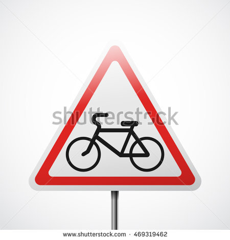
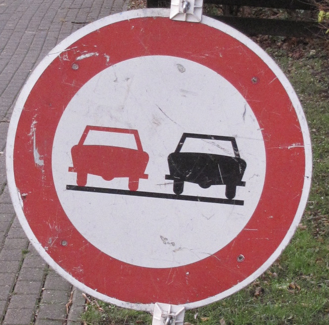
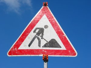
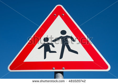
Here are five German traffic signs that I found on the web:
Bicycle crossing challenges: Writing across sign + white bar at bottom might be interpreted as a feature
No passing challenges: Rotated from horizontal
Turn straight or right challenges: Writing, X across sign
Road work challenges: Picture taken from low angle
Children crossing challenges: Picture taken from low angle + writing across sign + white bar at bottom
All five images were not quite square. In resizing and interpolating them down to 32x32 squares, their aspect ratios are skewed. This may also prove a challenge for the network.
2. Discuss the model's predictions on these new traffic signs and compare the results to predicting on the test set. At a minimum, discuss what the predictions were, the accuracy on these new predictions, and compare the accuracy to the accuracy on the test set (OPTIONAL: Discuss the results in more detail as described in the "Stand Out Suggestions" part of the rubric).
Here are the results of the prediction:
| Image | Prediction |
|---|---|
| Bicycle crossing | Beware of ice/snow |
| No passing | No passing |
| Straight or right | Straight or right |
| Road work | Road work |
| Children crossing | Children crossing |
The model was able to correctly guess 4 of the 5 traffic signs, which gives an accuracy of 80%. Both the bicycle crossing sign and the beware of snow sign are red and white triangles with relatively delicate internal features containing crossed lines and circular patterns, so it is unsurprising that the network would confuse them. Also, bicycle crossing signs were relatively underrepresented in the initial (unaugmented) training set.
3. Describe how certain the model is when predicting on each of the five new images by looking at the softmax probabilities for each prediction. Provide the top 5 softmax probabilities for each image along with the sign type of each probability. (OPTIONAL: as described in the "Stand Out Suggestions" part of the rubric, visualizations can also be provided such as bar charts)
The cell Output Top 5 Softmax Probabilities For Each Image Found on the Web of the jupyter notebook or html output contains my code for outputting softmax probabilities for each image from the web. The top five softmax probabilities for each image are listed, along with bar charts.
For the no passing, straight or right, and road work signs, the model is very (>99%) certain.
For the bicycle crossing sign, the network is less certain (73%) of its incorrect "Beware of ice/snow" guess. It believes the sign may also be a road work sign (13.7%) or bicycle crossing sign (9.3%).
For the children crossing sign, the model is only 52% certain, and believes the sign may be a bicycle crossing sign with 47.6% probability. This is unsurprising because these two sign types are visually similar.
Please refer to the jupyter notebook or html output for more information.


