This project implements an unscented Kalman filter in C++.
Input data consisting of lidar measurements (given directly as x and y positions, with some known uncertainty) and radar measurements (given as radius, angle, and radial velocity relative to some fixed measurement site, with some known uncertainty) are combined with a motion model to track a vehicle with much better accuracy than the individual measurements alone allow.
The code presented here is designed to work with the Udacity term 2 simulation executable, and so cannot be run standalone. However, here's some example output.
Red circles are lidar measurements. Blue circles are radar measurements (position markers inferred from radius and angle; the also-supplied radial velocity measurements are not shown). Green markers are the car's position as estimated by the Kalman filter.
In this project, I used a "constant turn rate and velocity magnitude" (CTRV) process model to carry out the Kalman filter's predict steps. The CTRV tracks a state vector of 5 quantities: x position, y position, velocity magnitude, yaw angle, and yaw rate. To predict the position from the time of the old measurement to the time of the current measurement, the velocity magnitude and yaw rate are assumed to be constant; however, a random linear (in the direction of the velocity) acceleration and yaw acceleration are assumed to exist at each time interval. Both accelerations are uncorrelated with a mean of zero and a constant variance.
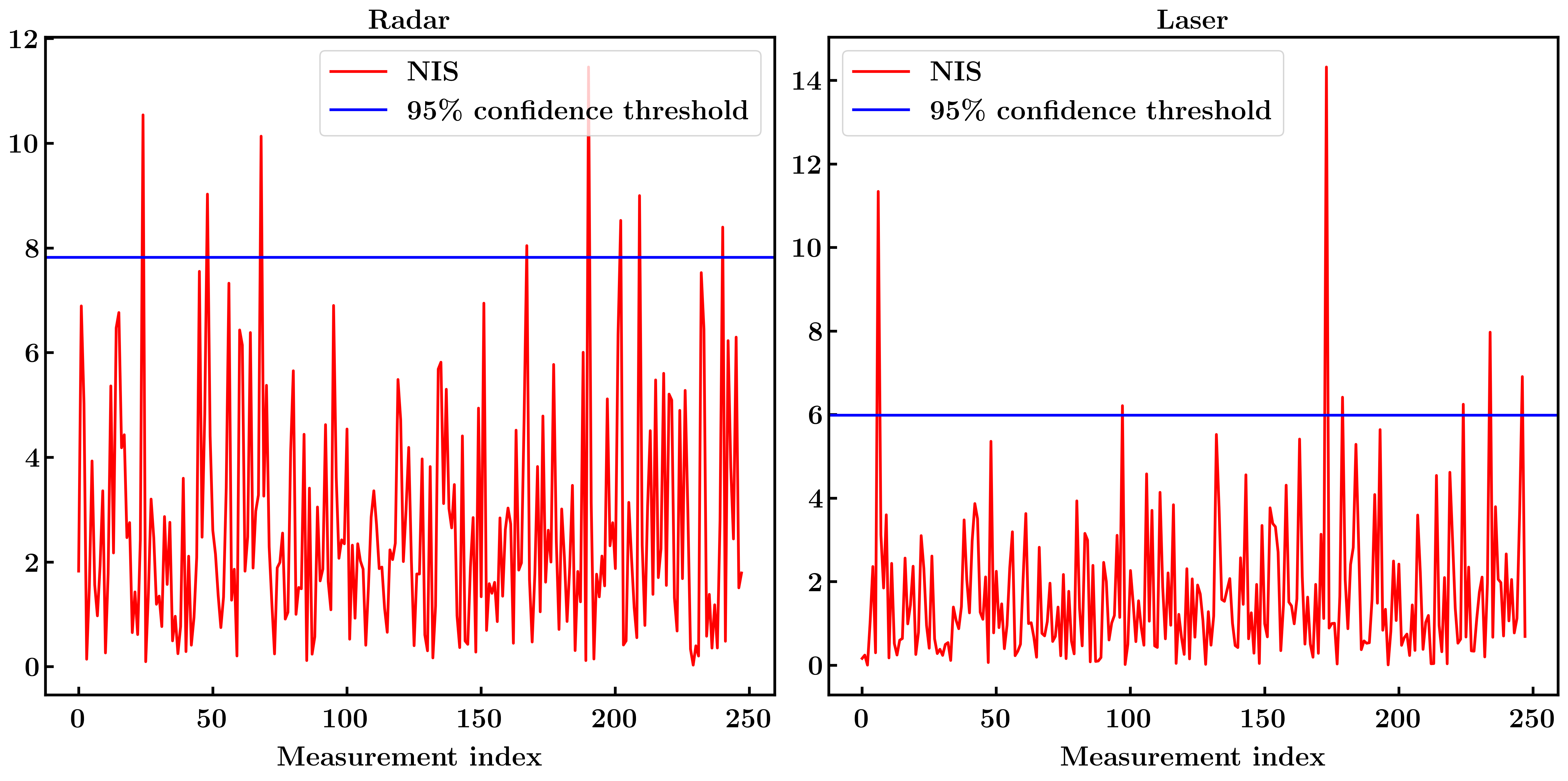
Part of this project was choosing the hardcoded variance of the random linear and yaw rate accelerations applied during the predict step. The chosen values should be physically reasonable (i.e., a bike or car will not abruptly accelerate at 100 m/s^2, so the variance should be significantly less than 100^2). A good way to check if the noise values are physically reasonable is to use the "normalized information squared" or NIS statistic. If our chosen variances used in the prediction step are consistent with physical reality, the NIS values computed from the radar measurements should roughly obey a chi-square distribution with degrees of freedom equal to the dimension of the radar measurement space (3). Similarly, NIS values computed from the laser measurements should roughly obey a chi-square distribution with 2 degrees of freedom. A concrete heuristic way to check this is to plot the NIS statistic for the radar or lidar measurements along with the corresponding 95% confidence threshold of the chi-square distribution, which is 7.82 for 3 degrees of freedom (radar) and 5.99 for 2 degrees of freedom (lidar). If our noise is consistent, we should see roughly 95% of NIS values computed from measurements fall below that confidence threshold, which appears just about right for my chosen process noise variances (9 m^s/s^4 for the linear acceleration and 1 rad^2/s^4 for the yaw rate acceleration):
Maybe a few more NIS samples should exceed the threshold (particularly for laser measurements) but I'm satisfied for now. If I wanted to fine tune forther, the NIS statistic could be used to adjust the process noise as follows:
If much more than 5% of the NIS values computed from measurements exceed the threshold, it means that our measurements are actually being drawn from a distribution with a greater variance than we assumed. In other words, we have underestimated the process noise, and should increase it.
If all of the NIS values computed from measurements fall well below the threshold, it means that our measurements are being drawn from a distribution with smaller variance than we assumed. In other words, we have overestimated our process noise, and should decrease it.
