This short package provides fast estimation of the estimators of agreement for multiple observers. The data are assumed to include a matrix or data-frame with subjects as the rows and observers as the columns, with nominal or ordinal categories as the data. The methods are described by O’Connell and Dobson (Biometrics 1984; 40: 973-983) and Schouten (Statistica Neerlandica 1982: 36: 45-61).
There are several estimators of particular interest here:
- O’Connell-Dobson-Schouten estimator of average agreement across the observers.
- Average agreement by subject (O’Connell and Dobson 1984)
- Average agreement by observer (Schouten 1982)
P-values compared with the null hypothesis (that is, H0: average agreement is zero) are available for these estimators. For the average agreement by observer, p-values are also available compared with the average agreement across observers.
The summary methods describe a range of estimators, including confidence intervals. Several plots are available.
The Fortran code from O’Connell and Dobson was provided by Professor O’Connell. The algorithms described by Schouten (1982) were implemented in Fortran 77.
Both O’Connell and Dobson (1984) and Schouten (1982) use the data from Landis and Koch (Biometrics 1977; 33: 363-374). The data are included as the landis dataset in the R package.
A simple description of the average agreement across the observers is given by printing the magree object:
require(magree)
magree(landis)
#+RESULTS[3f3328a44897fea629d021aa38d85d7da20e960f]:
O'Connell-Dobson-Schouten estimator (unweighted)

Sav(hetero):	0.361290 (se: 0.028881; 95% CI: 0.306811, 0.419587)
Sav(homoge):	0.354335 (se: 0.030018; 95% CI: 0.297924, 0.415112)
Pr(Overall agreement due to chance | hetero):	< 2.22e-16
Pr(Overall agreement due to chance | homoge):	< 2.22e-16
We can obtain considerably more information from the summary of the magree object:
summary(magree(landis))#+RESULTS[fa757baf5e4f9c8efde3a95f84b1890b0ca98e41]:
O'Connell-Dobson-Schouten estimator (unweighted)

Sav(hetero):	0.361290 (se: 0.028881; 95% CI: 0.306811, 0.419587)
Sav(homoge):	0.354335 (se: 0.030018; 95% CI: 0.297924, 0.415112)
Pr(Overall agreement due to chance | hetero):	< 2.22e-16
Pr(Overall agreement due to chance | homoge):	< 2.22e-16

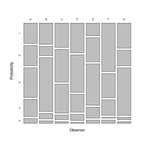
Observed marginal distributions for categories:

         1          2          3          4          5
0.28087167 0.25423729 0.36440678 0.07384988 0.02663438

Observed marginal distributions for categories by observer:

          1         2         3           4           5
A 0.2203390 0.2203390 0.3220339 0.186440678 0.050847458
B 0.2288136 0.1016949 0.5847458 0.059322034 0.025423729
C 0.2627119 0.3559322 0.3135593 0.050847458 0.016949153
D 0.3220339 0.4067797 0.1949153 0.067796610 0.008474576
E 0.1355932 0.2627119 0.4491525 0.118644068 0.033898305
F 0.5254237 0.2627119 0.1694915 0.008474576 0.033898305
G 0.2711864 0.1694915 0.5169492 0.025423729 0.016949153

Agreement statistics S_i for each subject:

          1           2           3           4           5           6
 0.08088076  1.00000000  1.00000000  0.34348626  1.00000000  0.34348626
          7           8           9          10          11          12
 0.60609175  0.21218351  0.27783488  0.60609175  0.60609175  0.60609175
         13          15          16          17          18          19
 0.60609175  0.21218351  0.08088076  0.60609175  0.21218351  0.21218351
         22          23          24          25          26          27
 0.08088076  0.60609175  0.34348626  0.34348626  1.00000000  0.34348626
         28          29          30          31          32          33
 0.08088076  0.34348626  0.60609175  1.00000000  0.27783488  1.00000000
         34          35          36          37          38          39
 1.00000000  0.27783488  0.27783488  0.08088076  0.01522939  0.34348626
         40          41          42          43          44          45
 0.08088076  0.60609175  1.00000000  0.08088076  0.27783488  0.60609175
         46          47          48          49          51          52
-0.05042199  0.21218351  0.34348626  0.08088076  0.60609175  0.27783488
         53          54          55          56          57          58
 0.27783488  0.01522939  0.60609175  0.60609175  0.01522939  1.00000000
         59          60          61          62          63          64
 1.00000000  0.60609175  0.08088076  0.27783488  0.08088076  0.21218351
         65          66          67          68          69          70
 0.60609175  0.08088076  1.00000000  0.34348626  0.27783488  1.00000000
         71          72          73          74          76          77
 0.60609175  0.27783488  0.60609175  0.01522939  0.60609175  0.34348626
         78          79          80          81          82          83
 0.08088076  0.34348626 -0.11607336  1.00000000  0.21218351  0.08088076
         84          85          86          87          88          89
 0.27783488 -0.18172474  0.60609175  0.60609175  0.01522939 -0.11607336
         90          91          92          93          94          95
 0.08088076  0.01522939 -0.11607336  0.21218351  0.34348626  0.27783488
         96          98          99         100         101         102
-0.11607336  0.21218351  0.21218351  0.08088076  0.34348626  0.34348626
        103         104         105         106         107         108
 1.00000000  0.01522939  0.60609175  0.08088076  0.21218351  0.08088076
        110         111         112         113         114         115
 0.21218351  0.60609175  0.21218351  0.08088076  0.08088076  0.21218351
        116         117         118         119         120         121
 0.60609175  0.34348626  0.08088076  0.60609175  1.00000000  0.21218351
        122         123         124         126
-0.11607336 -0.11607336  0.60609175  0.01522939

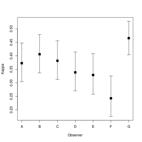
Agreement statistics for each observer:

    Kappa [Lower, Upper] Pr(kappa_av=kappa_observer)
A 0.37274 0.30394 0.4471                     0.60718
B 0.40591 0.33691 0.4788                     0.03444 *
C 0.38173 0.31292 0.4556                     0.40306
D 0.33866 0.27026 0.4145                     0.33175
E 0.32894 0.25801 0.4086                     0.23888
F 0.24269 0.17536 0.3257                     < 1e-05 ***
G 0.46538 0.40385 0.5280                     < 1e-05 ***
---
Signif. codes:  0 ‘***’ 0.001 ‘**’ 0.01 ‘*’ 0.05 ‘.’ 0.1 ‘ ’ 1
There are currently two plot types: the default type = “p1” gives a tabular plot for the marginal probabilities of each category by observed:
plot(magree(landis))#+RESULTS[ac7ce3b55597642e6c75f253cad009bda11d8338]:

The second plot is type = “kappa by observer”, which shows the estimated average kappa by observer with intervals based on single standard errors:
plot(magree(landis),type="kappa by observer")#+RESULTS[8172ce7d6a34ee663adfe7d6e788b083b17c67f2]:

- Better describe the difference between the estimators that assume homogeneity and those that assume heterogeneity.
- For the average agreement by subject, calculate p-values compared with the average agreement across subjects (which equals the average agreement across observers). This will require an estimate of the covariance between the average agreement across subjects and the average agreement by subject. As the code is so fast, it may be possible to calculate these values using the jackknife or similar approach.
- Extend the O’Connell-Dobson estimators to include an arbitrary weight matrix.