Systematic analysis of dark and camouflaged genes
We present a list of dark and camouflaged genes and .bed files specifying their genomic coordinates. We provide scripts on how these regions were defined and a pipeline on how to rescue variants from these regions in short-read data.
Check out our paper, here.
What are dark genes?
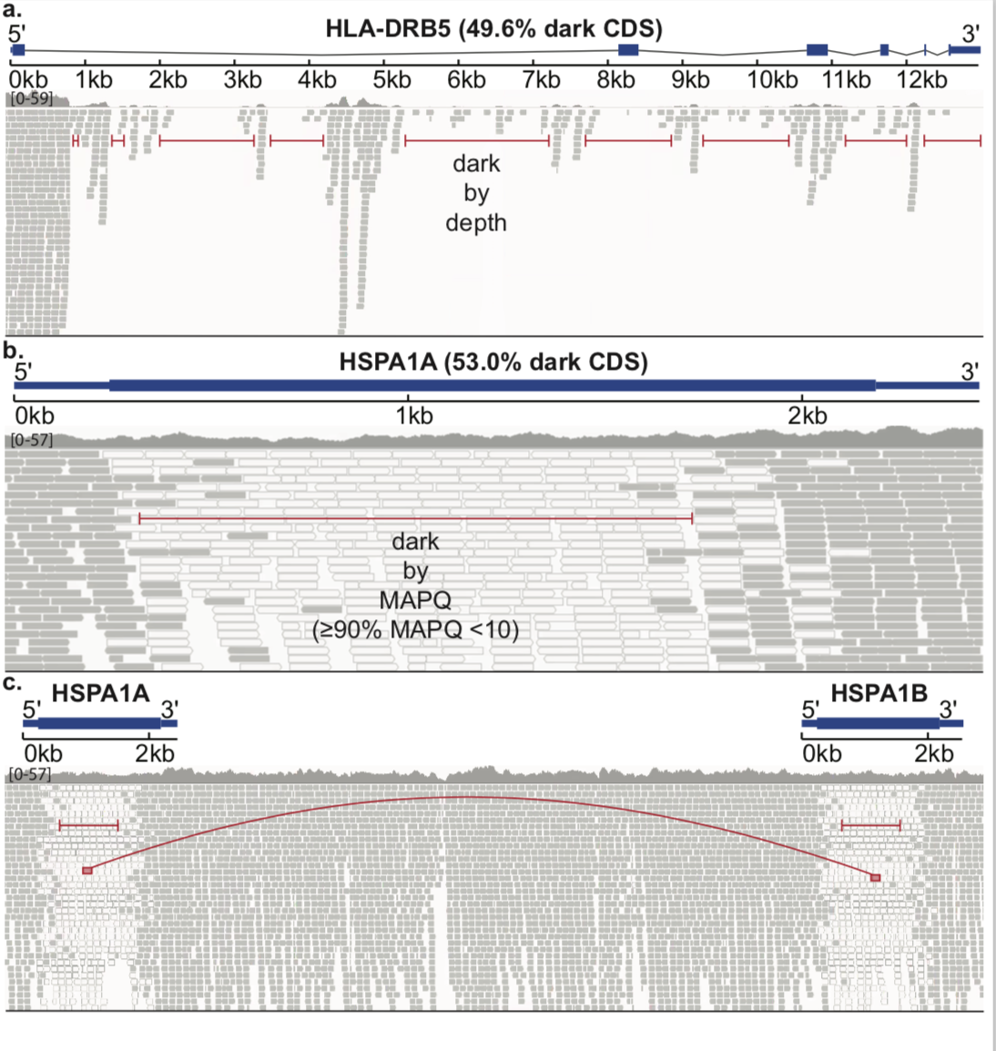
Dark regions of the genome are those that cannot be adequately assembled or aligned using standard short-read sequncing technologies, preventing researchers from calling mutations in these regions. We define two subclasses of dark regions: 'dark by depth' (where ≤ 5 reads map to the region) and 'dark by MAPQ' (where reads align but ≥ 90% of reads have MAPQ < 10). A specific subset of dark by MAPQ genes are camouflaged genes, dark genes that are the result of duplication events in the genome.
The IGV pile-ups above show examples of these dark regions. a) HLA-DRB5 is dark by depth, because no reads align to this region. b) HSPA1A is dark by MAPQ because reads align, but all the reads that do have poor MAPQ and would be filtered out by variant callers. c) The reason HSPA1A is dark by MAPQ is because of a gene duplication event: it is camouflaged by HSPA1B. The two genes are nearly identical so aligners can't determine from which gene a read originated.
We discovered dark regions are increasingly prevelant across the human genome. Based on standard whole-genome Illumina sequencing data, we identified 36794 dark regions in 6054 gene bodies (3804 protein-coding) from pathways important to human health, development, and reproduction. Of the 6054 gene bodies, 527 (8.7%) were 100% dark (117 protein-coding) and 2128 (35.2%) were ≥5% dark (592 protein-coding). We found 2855 dark regions were in protein-coding exons (CDS) across 748 genes. Many of these genes are important to human health and disease.
We have also developed an algorithm to resolve most of these camouflaged regions in short-read data. Here we apply it to the Alzhiemer's Disease Sequencing Project (ADSP) whole exome case control study. We provide the scripts we used to characterize these regions and apply our algorithm to ADSP.
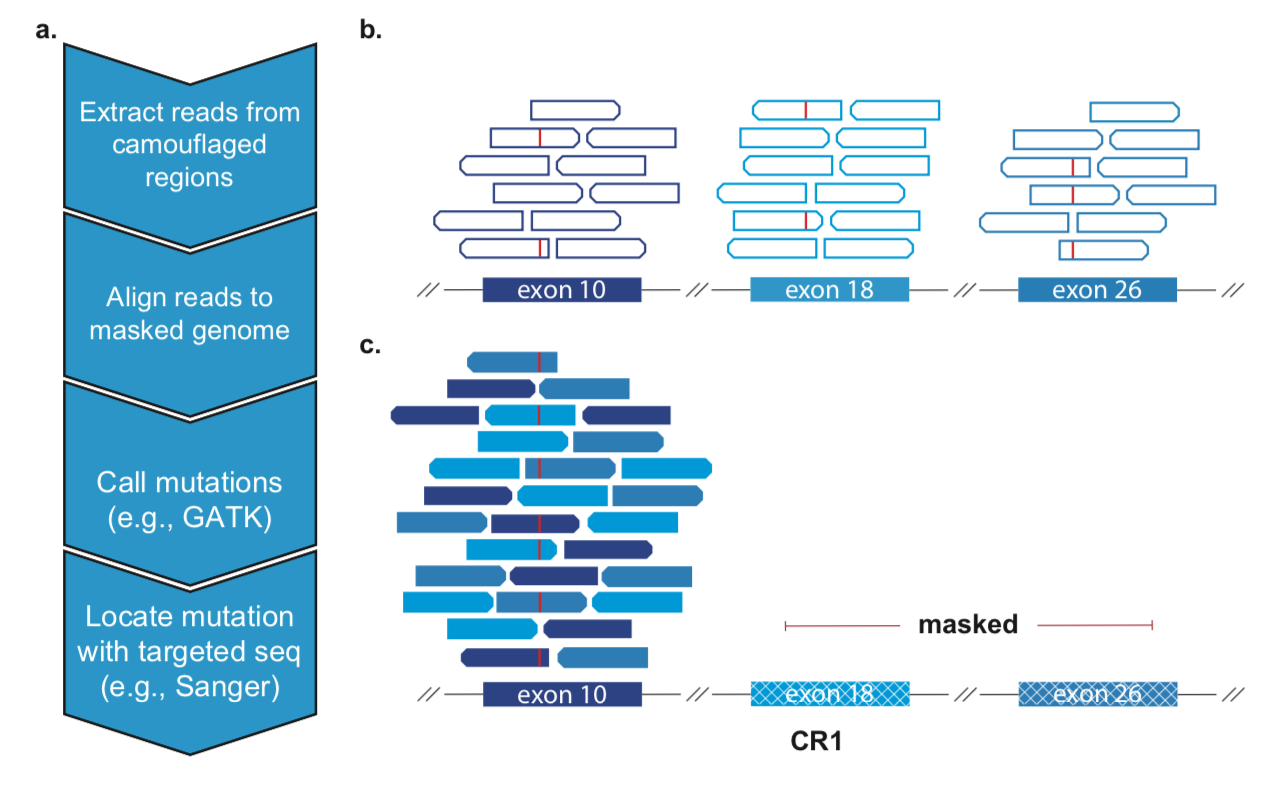
As a proof of concept, we used these methods to find a variant in ADSP present in 5 Alzhiemers Disease cases, but 0 controls in the CR1 gene (a top AD gene that is also 26% dark CDS )
Running our analysis
We have divided up our scripts into 11 distinct steps found in the scripts directory. These steps can broadly be placed into 3 categories. 1. Steps 00-05 are used to caracterize dark regions and create the .bed files used in our analysis pipeline. 2. Steps 06-10 contain the scripts we used to call camo variants in ADSP. Finally, 3. step 11 contains all the scripts used to plot figures for our manuscript.
Each step should be self contained, but may depend on the output of previous steps. With in each step directory there is a submit.sh script, that will automate the running of all the scripts for that step. At the top of the submit script is an in-depth description of what each step is doing, as well as a list of entry points required for that step. Before running a submit.sh script be sure to update the entry points at the beginning of that script.
A brief outline of each step is summarized below:
-
00_GET_BAMS Scripts used to align Fastq reads from 10X and ONT and to realign all bams to the three different genome builds (b37, hg38, hg38+alt).
-
01_RUN_DRF Scripts used to run the DarkRegionFinder on the bams. In brief, walks through the genome and for every base prints the read depth and mass of reads with low MAPQ.
-
02_COMBINE_DRF_OUTPUT Scripts used to average together the DRF output from the 10 illumina samples and split the combined output into a dark_by_depth bed file and a dark_by_mapq file.
-
03_CALC_BAM_METRICS Scripts used to calculate the median coverage and read lengths for all the sequencing technologies.
-
04_PREPARE_ANNOTATION_BED Bedtool arithmetic scripts to convert Ensembl GFF3 annotation file from transcript level to a gene level annotation (condensing multiple transcripts). As well as removing overlapping annotations or genes.
-
05_CREATE_BED_FILE Uses the split DRF output from step 2 and intersects it with the annotation bed from step 4 to quanitfy just how dark gene bodies are. Produces the supplemental tables shown in our manuscript. Also blats the low_mapq dark regions and maps them to eachother to create camouflaged .beds that will be used in our camo variant rescue pipeline.
-
06_MASK_GENOME Uses the camo align_to file from step 5 to create a camo masked genome.
-
07_RUN_ADSP Scripts to realign camo reads from the ADSP exome bams and realign them to the camo-masked genome from step 6, and then call variants in these regions.
-
08_COMBINE_AND_GENOTYPE_ADSP Takes the intermediate gVCFs from step 7 and combines and genotypes them.
-
09_FIND_FALSE_POSITIVES Creates a bed file listing positions in the camo-masked genome where reference-based artifacts might be called.
-
10_VARIANT_FILTERING Combines the VCFs from step 8 and annotates the VCF with inbreeding coefficient. Filters out variants present in the reference-based artifact bed created in step 9 and that have low QD values.
-
11_FIGURES Rmarkdown scripts we used to plot all the figures for our manuscript .
Using our camouflaged .bed files
We encourage researchers to use our methods and the provided .bed files to call camo variants within their own data sets.
We outline our short-read data pipeline to rescue camo variants below:
We provide two .bed files to define and call variants in camouflaged genes. The .bed files were created from 10 whole genomes generated with Illumina paired-end read Sequencing with a 100bp read length. The realign .bed file defines all gene-body elements (i.e. exon, intron, UTR, etc.) that contain a camo region and which other gene-body element(s) share high sequence identity which causes the regions to camouflage eachother. The fourth column of the realign .bed file contains a semi-colon delimited list of gene-body element IDs. The first ID corresponds to the given genomic position, while all subsequent region IDs are regions with high sequence identity that are camouflaged together. The realign file is used as an argument to samtools view to extract all low-MAPQ reads that fall within camouflaged genes. The entire gene-body element is used in the realign file as opposed to just the camouflaged region in order to potentially capture more variants in flanking sequences (which tend to be highly homologous yet failed to meet our strict cutoffs).
The alignto .bed file is similar to the realign .bed file, but it only contains the coordinates for one gene-body element per camoulog group. For example, CR1 exons 10, 21, and 26 are nearly identical and are all camouflaged to eachother. The realign .bed will contain the coordinates for all three exons, while the alignto .bed will only contain coordinates for exon 10. Thus, the alignto file defines which repeated region will be used to align the extracted reads, and which repeated regions will be masked. The complement of the alignto .bed is used to mask the genome. When masking the genome, each region in the alignto .bed is expanded by 50bp so that reads extracted near the boundary of a camo region can accurately align.
The final column of the alignto and realign .bed lists the repeat number of the camoulog group--the number of times this sequence appears in the genome with high homology. We recommend only calling variants in regions with ≤ 5 repeat number. Depending on this repeat number we also call variants using GATK with different ploidies. Variants within a region where the camoulog group repeat number of 2, are called with a ploidy of 4. Whereas in the CR1 example, we would use a HaplotypeCaller ploidy of 6.
The GATK.bed provided is essentially the same as the align_to.bed with the exception that it is restricted to CDS regions and only lists the interval of that actual camo region and not the whole gene body. The GATK.bed is passed into GATK to define the interval over which to call variants. We only called variants strictly in camo regions and only in CDS regions to avoid calling too many false positives.
In order to use these .bed files to call camouflaged variants in your own data set, follow the scripts found in the steps 06_CREATE_BED_FILE to 10_VARIANT_FILTERING directories. A brief outline of the workflow is as follows:
For each repeat number to be tested (we recommend ≤ 5), do the following:
-
Expand the alignto .bed file by 50 and use it to mask the genome for this ploidy
-
Use the realign .bed file to extract reads from the correct repeat number regions
-
Align these reads to the new camo masked reference with bwa mem
-
Use GATK HaplotypeCaller to call variants specifying the correct ploidy and setting the interval to the GATK .bed
-
Combine and Genotype gVCF files across the whole cohort to create the ploidy specific VCF
-
Filter out false positive variants with QD and InbreedingCoeff cutoffs and remove variants found in reference-based artifact positions
-
Convert polyploid VCFs to diploid and use plink2 to test associations
Any variants found using these methods should be investigated independentally and then experimentally validated to ensure they are not false positives and then to determine in which specific camouflaged region the variant actually lies.

