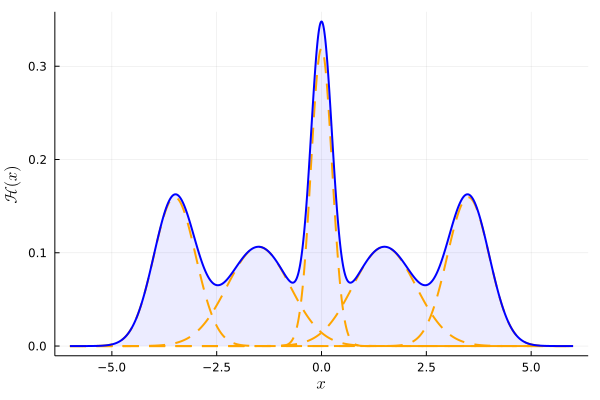
A lightweight Julia package to plot a density function for a given set of values with known uncertainties.
An example application of the main exported abstract struct, ContinuousHistogram, is to visualize a "histogram" of experimental values, when each value has a measured experimental uncertainty. This is to be contrast with normal Histogramming that assumes that each value is exact, meaning its uncertainty is zero().
This package provides similar functionality to what is expected from kernel density estimation (KDE), but here the data errors/uncertainties which act as the kernel bandwidths are all, in principle, different.
An example GaussianHistogram <: ContinuousHistogram can be constructed from the following Julia code
using Plots # One must Pkg.add this separately
using UncertainHistogramming
Plots.gr()  # Use GR to reproduce the plot exactly

# Create a list of (value, error)-tuples
values_errs = [(-3.5, 0.5), (-1.5, 0.75),
               (0, 0.25), (1.5, 0.75),
               (3.5, 0.5)]

# Initialize the GaussianHistogram and
# push! the data into it
hist = GaussianHistogram()
push!(hist, values_errs)

# Create an argument array to build the
# ContinuousHistogram from
x = LinRange(-6, 6, 3000)

# Plot using a User Recipe
# (thanks to RecipesBase.jl)
plot(x, hist)

