plawt - JSON-like sugar for matplotlib

Because sometimes you just want a good looking plot damnit. I don't like context switching from physics to python, and hopefully this will let me do less of it.

Installation

pip install plawt and then import plawt in your python file. Current version is here.

Features

See the examples folder for how to use plawt to make subplots, step plots, and other less common uses.

In addition to any usual single panel plot plawt also wraps these matplotlib features:

Arbitrary subplot grids, spacing between subplots
Step Plots
Log plots
legends, legend locations, legend labels
labelling, subplot titles (with location), super titles, font-size tweaking
x limits, y limits,
marker and linestyle, alpha, drawstyle
saving figures, showing figures to screen
tight_layout
matplotlib style (plt.style.use())
Tick parameters (axes.tick_params)
Text annotations

Example

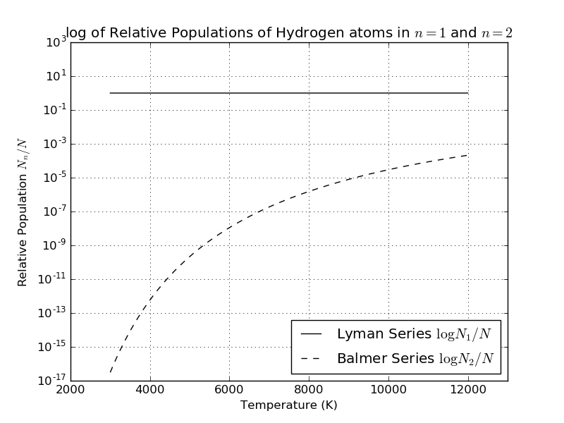
Here's a simple logarithmic plot that shows why the strength of Balmer lines varies in different colored stars:

Here's the code for that plot using plawt:

from __future__ import division
from math import pi
from numpy import exp, sqrt, log10, e
import numpy as np
import plawt

### Functions to generate the data
# excitation potential
def Xn(n): return 13.6*(1-1/n**2)

# Boltzmann equation, N_n/N
def excitationEq(n, T):
	k = 8.63e-5 # eV/K
	gn = 2*n**2; Z = 2 # hydrogen atom
	return (gn/Z) * exp(-Xn(n)/(k*T))

T = np.arange(3000, 12000, 1)

### now all the data and metadata about the plot:
myplot = {
	0: {	# 'first' line
		'x': T,
		'y': excitationEq(1, T),
		'line': 'k-',
		'label': 'Lyman Series $\log{N_1 / N}$'
	},
	1:{		# 'second' line
		'x': T,
		'y': excitationEq(2, T),
		'line': 'k--',
		'label': 'Balmer Series $\log{N_2 / N}$'
	},
	'xlabel': 'Temperature (K)',
	'ylabel': 'Relative Population $N_n / N$',
	'title': 'log of Relative Populations of Hydrogen atoms in $n=1$ and $n=2$',
	'set_yscale': 'log',
	'grid': True,
	'legend': {'loc':4},
	'ylim': (10e-18, 10e2),
	'xlim': (2000,13e3),
	'filename': 'excitation_logarithmic.png',
	'show': True
}

### fire away fire awaaay
plawt.plot(myplot)

The plot is also saved. I prefer this because I can glance at what is completely just information about the physical problem I'm working on. What are my labels? What is my data? What are my limits? Is it a log scale? Plus a few extra aesthetic things like grid, line color, the name of the file it's being saved as, etc.

The same plot above is written like this without plawt:

plt.plot(T, excitationEq(1, T), 'k-', label='Lyman Series $\log{N_1 / N}$')
plt.plot(T, excitationEq(2, T), 'k--', label='Balmer Series $\log{N_2 / N}$')
plt.xlabel('Temperature (K)'); plt.ylabel('Relative Population $N_n / N$')
plt.title('log of Relative Populations of Hydrogen atoms in $n=1$ and $n=2$')
plt.gca().set_yscale('log')
plt.legend(loc=4)
plt.grid()
plt.ylim((10e-18,10e2))
plt.xlim((2000, 13e3))
plt.savefig('excitation_logarithmic.png')
plt.close()

Usage

There is only one exposed method:

plawt.plot(plotDictionary)

You specify your plot in a python dictionary, here called plotDictionary. Each line (data series) in your plot should be indexed by an integer key. The actual integer doesn't matter but I like to go 0, 1, 2, ...

I define my data series before anything else.

plotDictionary = {
	0: {
		'x': [1, 2, 3, 4, 5, 6],
		'y': [1, 2, 3, 4, 5, 6],
		'line': 'k-' # black, solid, like in matplotlib docs
	}
}

The value of the '0'th line is another dictionary. The only mandatory fields are 'x' and 'y'. The 'line' field is optional as well as 'label'.

In fact every field except for a 'x' and 'y' is optional.

Note: Not every pyplot field is implemented! I add fields as I need them. Send me pull requests if you'd like something added.

I try to keep a one-to-one mapping between the fields in plawt and in matplotlib:

Add an xlabel the same way as in matplotlib:

plt.xlabel('numbers<3')

## OR ##

plotDictionary = {
	0: {
		'x': [1, 2, 3, 4, 5, 6],
		'y': [1, 2, 3, 4, 5, 6],
	},
	'xlabel': 'numbers<3'
}

The values of some fields also match with their matplotlib counterparts: eg. a log scale:

plt.gca().set_yscale('log')

## OR ##

plotDictionary = {
	0: {
		'x': [1, 2, 3, 4, 5, 6],
		'y': [1, 2, 3, 4, 5, 6],
	},
	'set_yscale': 'log'
}

By default plawt will close your plot automatically after showing it to you or saving it to a file. If you set 'keepOpen':True you can take the return value and use it to do more things to your plot that haven't been implemented yet:

plotDictionary = {
	0: {
		'x': [1, 2, 3, 4, 5, 6],
		'y': [1, 2, 3, 4, 5, 6],
	},
	'keepOpen': True
}

plt = plawt.plot(plotDictionary)
plt.gca(). etc etc
plt.savefig('yo.png')
plt.show

## Or even just
plawt.plot(plotDictionary).show()

MIT License

mef51/plawt

plawt - JSON-like sugar for matplotlib

Installation

Features

Example

Usage