Machine Learning Graduate Studies
The purpose of these notes are to
- Identify different types of machine learning problems
- Know what a machine learning model is
- Know the general workflow of building and applying a machine learning model
- Know the advantages and disadvantages about machine learning problems
Machine Learning Model
To start off, machine learning nowadays does not go beyond a computer program that performs the predefined procedures. What truly distinguished a machine learning algorithm from a non machine learning algorithm, such as a program that controls traffic lights, is its ability to adapt its behaviours to new input. This adaption seems to imply that the machine is actually learning. However, under the hood, this perceived adaption of behaviours is as rigid as every bit of machine instructions.
A machine learning algorithm is the process that uncovers the underlying relationship within the data. The outcome is called the machine learning model. The model changes when fed different data, meaning the function is not predefined and fixed.
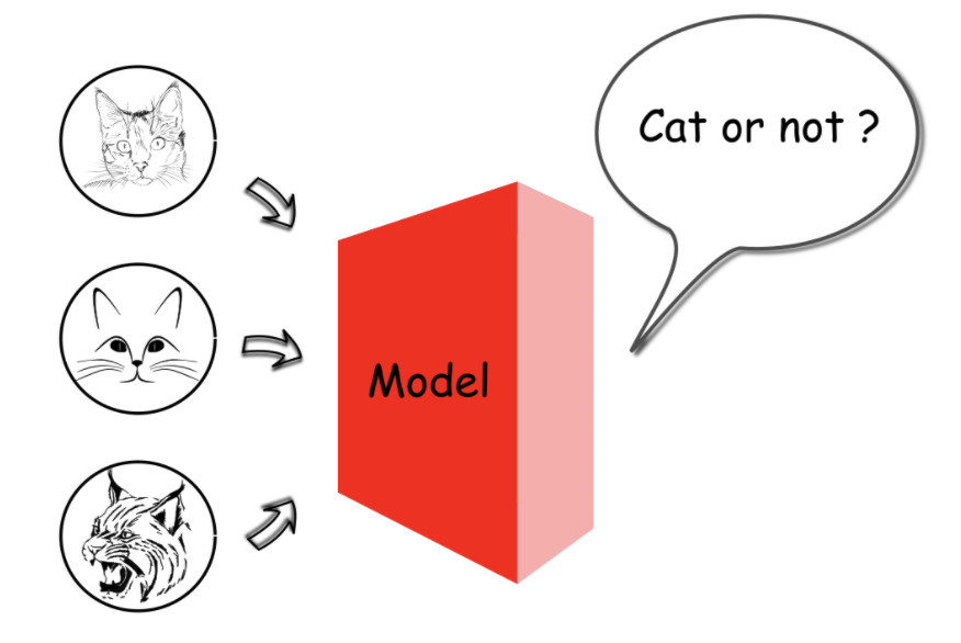
The input of the generated model here would be a digital photo, and the output is a boolean value indicating the existence of a cat in the photo.
The model for the above case is a function that maps multiple dimensional pixel values to a binary value. For example, assume we have a photo of 3 pixels, and the value of each pixel ranges from 0 to 255. The mapping space between the input and output would be (256 X 256 X 256) X 2, which is around 33 million. This task of learning the mapping might be daunting; however,
The task of machine learning is to learn the function from the vast mapping space
The results of the machine learning model is often not 100% accurate. Before the wide application of deep learning in 2012, the best machine learning model could only achieve 75% accuracy in the ImageNet visual recognition challenge.
Supervised VS. Unsupervised
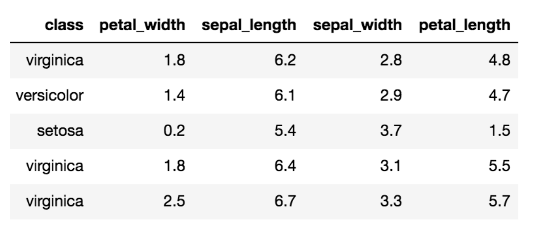
When first given a machine learning problem, one can determine whether it is a supervised or unsupervised problem. We start from a data set, which consists of a group of samples, and each sample can be represented as a tuple of attributes. A famous data set called Iris consists of different measurements for 150 samples of iris flower. Below is a sample of this data set:
Supervised Learning
There is a ground truth attribute for these models. This target attribute serves as a teacher to guide the learning task. It provides a benchmark on the results of learning. Hence, the task is called supervised learning. The class attribute (virginica, versicolor, setosa, etc...) of the iris dataset can server as a target attribute. The data with a target attribute is often called "labeled" data. We should now be able to determine that the task of predicting the category of iris flower with the labeled data is a supervised learning task.
Unsupervised Learning
An unsupervised learning task does not have the ground truth. We are expected to learn the underlying patterns or rules from the data without having the predefined ground truth as the benchmark. Here are a few examples:
- Clustering: one can cluster the samples from a data set into groups based on similarities among the samples within the data set. An example of clustering is a sample of a customer profiles and how many items were purchased or what time the customer visited the shopping site. After clustering customer groups together, one could devise commercial campaigns targeting each group.
-Association: uncovering the hidden association patterns among the attributes of a sample. A shopping cart of a customer could be seen as a sample, and each attribute of the sample is a piece of merchandise. Maybe we can derive that customers who bought beers often bought diapers as well.
Semi-supervised Learning
A data set might be massive but the labeled sample are few. In this case, we can apply both supervised and unsupervised learning. An example is how it took 2.5 years for the research team at Stanford to curate the famous ImageNet, which contains millions of images with thousands of manually labeled categories. Often is the case that one has a large amount of data, yet few of them are accurately "labeled". For example, videos without a category or even a title.
If only 10% of images in a data set are labeled, by applying supervised learning, we train a model with the labeled data. Next, we apply the model to predict the unlabeled data. This approach is not convincing; how general can this model be if we learnt from only a minority of the data set. Therefore, we first cluster the images into groups (unsupervised learning). Next, we apply the supervised learning algorithm on each of the groups individually. In this scenario, the unsupervised learning first narrows down the scope of learning so that the supervised learning in the second stage could obtain better accuracy.
Classification vs Regression
We can further distinguish the machine learning models as classification and regression based on the type of output values.
If the output of a machine learning model is discrete, such as a boolean value, then we call
it a classification model. A model that outputs continuous values is a regression model.
Classification Model
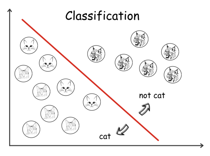
The model that tells whether a photo contains a cat or note can be considered as a classification model since the output is a boolean value:
A matrix M with dimensions of H x W where H is the height of the photo in pixels and W is the width of the photo can represent the input. Now, each element within the matrix is the grayscale value of each pixel in the photo, i.e. an integer value between [0,255] that indicates the intensity of the color. Again, the expected output of the model would be a binary value [1|0] that indicates whether the photo shows a cat or not. The formula can be formulated as follows:
F(M[H][W])=1∣0, where M[i][j]∈[0,255], 0<i<H, 0<j<W
The goal of machine learning is to discover the function that is as general as possible, which has a high probability to give the right answer for unseen data.
Regression Model
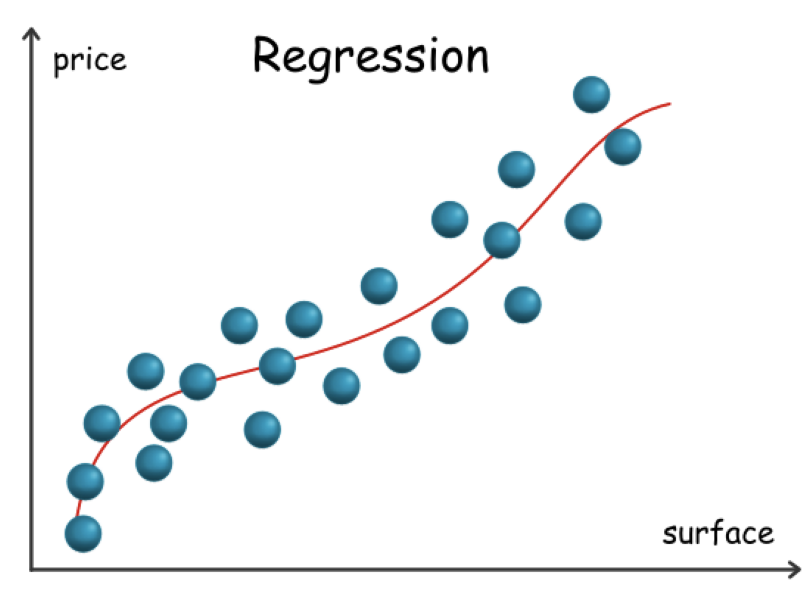
One can consider a model that estimates the price of real estate given the characteristics such as the surface, type type of real estate, and of course the location. We can expect the output as a real value p∈R; therefore, it is a regression model. Not all the raw data is numeric as some of them are categorical, such as the type of real estate. For each piece of real estate, we can represent its characteristics as a tuple T. The elements are also called features in many cases. The summary of the real estate model is as follows:
F(T)=p,where p∈R
If a piece of real estate were to have the following features:
surface = 120m^2, type = ' apartment', location = ' NY downtown', year_of_construction = 2000
If our model F was to return a value of $10,000, then we know it is not a good fit. The
following figure shows a model that takes only square footage as a variable.
 Some machine learning models like the decision tree can handle directly the non-numeric
feature as it is. More often, one has to transform those non-numeric features into
numeric one way or another.
Problem Conversion
Sometimes one can easily formulate a real world problem and quickly attribute it to either a classification or regression problem. The boundary between these two types of models might not always be clear, and one can transform a problem both ways.
The above example of real estate price estimation seems like a difficult prediction. What if we were to reformulate the problem to predict the price range of real estate instead of a single price tag? At this point, we can expect to obtain a more robust model. We have also transformed the model into a classification problem instead of regression.
The cat-photo-recognition model can also be transformed from a classification problem to a regression one. Defining the model to give a probability value of [0,100]% would do this transformation. If model B were to give a 49% probability while model A gave a probability of 1%, then we can tell that model B is closer to the truth. For this example scenario, one often applies one of the machine learning models called logistic regression, which gives continuous probability values as output. It is served to solve the classification problem.
Data, Data, Data!
The data ends up determining the upper bound of performance that the model can achieve. There are numerous models that can fit specific data, and the best we can do is to find a model that can closely approach this upper bound.
Rule of thumb: Garbage in, garbage out
In the example of four blind men who would like to conceptualize an elephant, none of the
four would get a full picture of what it looks like if they all only touched one part of
the animal.
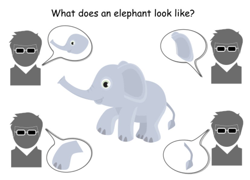
If the training data we received were only of those animal parts while the test processing data are full portraits of elephants, then we can expect our trained model to perform poorly. We do not have high quality data that is closer to the reality in the first place. This issue of gathering the data the captures the essential characteristics of the problem is a common struggle. One would not be able to learn anything from data that contains too much noise or is too inconsistent with the reality.
Machine Learning Workflow
What is the typical workflow to construct a machine learning model. One cannot talk about machine learning without mentioning the data. This relationship is as crucial as fuel to the engine of a rocket.
Data-Centric Workflow
The workflow to build a machine learning model is centralized around the data.
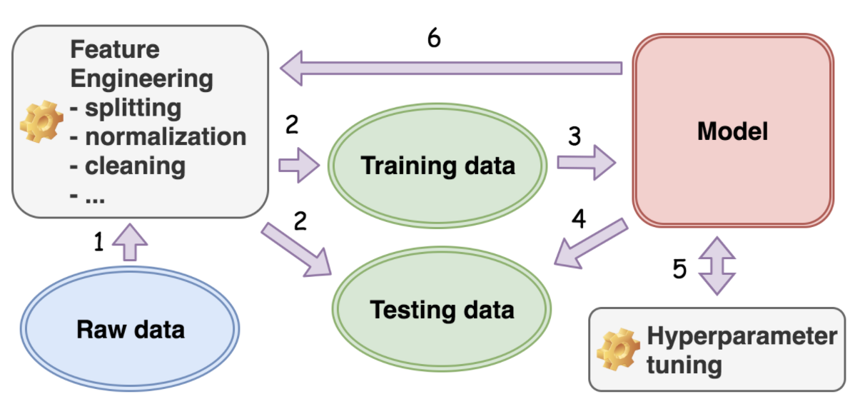
To say that the data dictates how the machine learning model is built is not exaggerating. A typical workflow involved in a project of machine learning is illustrated below:
We first determine which type of machine learning problems we would like to solve (i.e. supervised vs unsupervised). If the data is labeled, then one of the attributes in the data is the desired one, i.e. the target attribute. A boolean of yes|no for each cat photo could be an example of labeled data, which means it is a supervised learning problem.
Next, we determine the type of generated model: classification vs regression. This determination is based on the expected output of the model, i.e. discrete value for classification model and continuous value for the regression model.
After these determinations of the type of model we would like to build, we proceed with feature engineering, which is a group of activities that transform the data into the desired format. Examples of feature engineering are:
- Splitting* the data into two groups: training and testing. This practice is quite common, and the training dataset is used during the process to train a model. The testing dataset is then used to test or validate whether the model built is generic. Is the model generic enough that we can apply it to unseen data?
- Incomplete points in the dataset are also common. We might need to fill in those missing values with various strategies, one of which is just to fill with the average value.
- Encoding categorical attributes like county, gender, etc.. might be necessary due to the constraints of the algorithm. The linear regression algorithm can only deal with vectors of real values as input.
Feature engineering is not a one-off step; often one needs to revisit later in the
workflow.
After the data is prepares, we can select one of the machine learning algorithms and begin to feed the algorithms with the prepared training data. This process is called the training process.
Next, after the model is obtained at the end of the training process, it is then tested with the reserved testing data. This step is called the testing process.
After the first trained model, we will likely go back to the training process to tune some parameters. We call this hyper-parameter tuning, and it is called hyper because these parameters are the outermost interface that we interact with. These hyper parameters then have impacts on the underlying parameters of the model. For example, for the decision tree model, one of its hyper-parameters would be the maximum height of the tree. This parameters would limit the number of branches and leaves that a decision tree can grow at the end, which are the underlying parameters that a decision tree model consists of.
As you can decipher, the steps involved in the machine learning workflow form a cycle with
a focus on the data.
Underfitting vs. Overfitting
Two common cases for supervised learning algorithms (like classification and regression) is when the generated model does not fit the data well. An important measurement which we have mentioned before is generalization, which measures how well a model derived from the training data can predict the desired attribute of the unseen data. When we say that a model is underfitting or overfitting, it implies that the model does not generalize well to the unseen data. It is important to note that a model that fits well to the training data does not necessarily imply that it would generalize well to the unseen data. There are two reasons for this implication:
- The training data are just samples collected from the real world, which represents only a proportion of reality. The training data could simply not be representative.
- The data collected for the algorithm contains noise and errors. Then, the model that fits well with the training data would also capture the undesired noise and errors by mistake. This capturing would lead to bias and errors in the prediction for the unseen data.
In the task of classification, here is what underfitting and overfitting models look like:
Underfitting
An underfitting model is the one that does not fit well with the training data meaning it is significantly deviated from the ground truth. The model might be over-simplified for the data. In this case, the model may not be capable to capture the hidden relationships in the data. A simple linear line is not enough to clearly draw the boundary among the sample. Now, there is significant misclassification. We should then choose an alternative algorithm that is able to generate a more complex model from the training data.
Overfitting
This model will fit well with the training data to little or no error; however, it does not generalize well to the unseen data. A model that is able to fit every bit of data would fall into the traps of noises and errors. The figure above reveals less misclassification in the training data, yet it is more likely that this overfitted model would stumble on unseen data. We can try instead a simpler model for the training data. More commonly, one would keep the original algorithm that generated this overfitted model and add a regularization term. In a way, you are penalizing the model that is over-complicated so that the algorithm is steered to generate a less complicated model to fit the data.
Bias VS. Variance
Bias and variance are two terms that provide another perspective to the phenomenons of underfitting and overfitting.
Bias is a lerner's tendency to consistently learn the same wrong thing. Variance is the
tendency to learn random things unrelated to the real signal.
Let us first define the notion of main prediction before we dive deeper into bias and variance. The concepts of models and loss function are covered here.
Definitions
Given a training set s={(x1, t1), ... , (xn, tn)}, a learner, which is a machine learning algorithms, produces a model F. Now, given a test example xk, this model produces a prediction yk = F(xk). Each sample in the training set consists of two elements xi, which is a vector of attributes associated with the sample. ti is the target attribute to predict for the sample.
An example using these variables is as follows: xi = (type = "apartment", location = "LA", surface = "120m2"), ti = (price = "$420,000"). The task of a learner is to predict the price of an estate given its properties.
So, given a training sample (xi, ti), the learner produces a prediction as F(xi). The loss function L(F(xi),ti) is the difference between the prediction F(xi) and the true value ti associated with the sample. The larger the difference, the bigger the loss. The common loss function, square error, is adopted when a target attribute ti is of numerical value. This square error is defined as: L(F(xi), ti) = (F(xi) - ti)2. Following the above example, if the model F is to produce the price of the above example xi as "$410,000", then the result of the loss function would be (420,000 - 410,000)2 = 108.
Main Prediction
Given a loss function L and sets of training set S = {s1, s2, ..., sn}, the main prediction for a learner is defined as ym = argminy'Es(L(y,y')).
For each training set si, we train a model Fi with a given learner. Next, for a given training sample, we then produce a set of predictions Y = {y1, y2, ..., yn} with yi corresponding to the result produced by the model Fi. The main prediction ym is the prediction y' whose average loss with regards to all the predictions in Y is minimum. This definition means the main prediction is that which "differs least" from all the predictions in Y according to L.
Imagine the loss function is square error L(y, y') = (y - y')2. The main prediction with regards to the entire training set S is then the mean of the predictions, i.e. ym = Es(Y).
We can interpret the main prediction as the expected answer for a given training
sample from a given learner (a machine learning algorithm).
Now let's continue with an example -- a dart-throwing game where a learner is a player. Whenever a dart is thrown, the corresponding activities occur:
- The player poses and aims, meaning the learner trains a model from a given training dataset.
- The player throws the dart, meaning the model trained by the learner produces a prediction.
The bullseye is the target of the prediction, and the closer the dart is to the bullseye, the better the learner (player) is.
Before each throw, we can ask ourselves, "How many points will this player score?" The best guess we can take is the main prediction of this learner, which will in fact be the average score that the player has achieved during all past games.
Intuitively, we can consider that the main prediction is the general tendency (performance)
of a learner, i.e. expected points that a player can score in a game.
Let's now dive deeper into the concepts of bias and variance.
Bias
The phenomenon of underfitting and overfitting are explored more in the notions of bias and variance.
Bias is a learner’s tendency to consistently learn the same wrong thing. Variance is the tendency
to learn random things unrelated to the real signal.
Definitions
Given a training set S = {(x1,t1), ..., (xn,tn)}, a learner produces a model F. Given a test example xk, this model produces a prediction yk = F(xk). Each sample in the training set consists of two elements, xi, is a vector of attributes associated with the sample, and ti is the target attribute to predict for the sample.
To illustrate these definitions above, a train sample might look like xi = (type = "apartment", location = "LA", surface = "120m2"), ti = (price = "$420,000"). The task of a learner (again, a machine learning algorithm) is then to predict the price of an estate given its properties.
So, given a training sample (xi, ti), the learner produces a prediction F(xi), we then define the loss function L(F(xi), ti) as the cost that is incurred by the difference between the prediction F(xi) and the true value ti associated with the sample. Therefore, the larger the difference, the bigger the loss. A simple example of how to calculate the loss function is if the target attribute ti is of numerical value. Square error would be used here, and this formula looks like: L(F(xi), ti) = (F(xi) - ti)2. An example of square error in practice is if a model F produces the price of the above example xi as $410,000, then the result of the loss function would be (420,000 - 410,000) 2 = 108.
